curatedMetagenomicData
Lucas Schiffer, MPH
Section of Computational Biomedicine, Boston University School of Medicine, Boston, MA, U.S.A.schifferl@bu.edu
Levi Waldron, PhD
Graduate School of Public Health and Health Policy, City University of New York, New York, NY, U.S.A.levi.waldron@sph.cuny.edu Source:
vignettes/curatedMetagenomicData.Rmd
curatedMetagenomicData.RmdAbstract
The curatedMetagenomicData package provides standardized, curated human microbiome data for novel analyses. It includes gene families, marker abundance, marker presence, pathway abundance, pathway coverage, and relative abundance for samples collected from different body sites. The bacterial, fungal, and archaeal taxonomic abundances for each sample were calculated with MetaPhlAn3, and metabolic functional potential was calculated with HUMAnN3. The manually curated sample metadata and standardized metagenomic data are available as (Tree)SummarizedExperiment objects.
What curatedMetagenomicData provides
curatedMetagenomicData provides processed data from
whole-metagenome shotgun metagenomics, with manually-curated metadata,
as integrated and documented Bioconductor TreeSummarizedExperiment
objects or TSV flat text exports. It provides 6 types of data for each
dataset:
- Species-level taxonomic profiles, expressed as relative abundance
from kingdom to strain level (
relative_abundance) - Presence of unique, clade-specific markers
(
marker_presence) - Abundance of unique, clade-specific markers
(
marker_abundance) - Abundance of gene families (
gene_families) - Metabolic pathway coverage (
pathway_coverage) - Metabolic pathway abundance (
pathway_abundance)
Types 1-3 are generated by MetaPhlAn3; 4-6 are generated by HUMAnN3 using the UniRef90 database.
Currently there are:
- 22588 samples from 93 datasets; see the list of available studies
- 141 fields of specimen metadata from original papers, supplementary files, and websites, with manual curation and automated syntax-checking to standardize annotations
Installation
To install curatedMetagenomicData from Bioconductor, use BiocManager as follows.
if (!require("BiocManager", quietly = TRUE))
    install.packages("BiocManager")

BiocManager::install("curatedMetagenomicData")
Most users should simply install curatedMetagenomicData
from Bioconductor. Developers may install the GitHub repository with
remotes::install_github and the latest Bioconductor
development version.
R Packages
To demonstrate the functionality of curatedMetagenomicData, the dplyr and DT packages are needed.
Sample Metadata
The curatedMetagenomicData
package contains a data.frame, sampleMetadata,
of manually curated sample metadata to help users understand the nature
of studies and samples available prior to returning resources. Beyond
this, it serves two purposes: 1) to define study_name,
which is used with the curatedMetagenomicData() function to
query and return resources, and 2) to define sample_id,
which is used with the returnSamples() function to return
samples across studies.
To demonstrate, the first ten rows and columns (without any
NA values) of sampleMetadata for the
AsnicarF_2017 study are shown in the table below.
Data Access
There are three main ways to access data resources in curatedMetagenomicData.
- The
curatedMetagenomicData()function to search for and return resources. - The
returnSamples()function to return samples across studies. - Through the curatedMetagenomicDataTerminal command-line interface.
curatedMetagenomicData()
To access curated metagenomic data, users will use the
curatedMetagenomicData() function both to query and return
resources. The first argument pattern is a regular
expression pattern to look for in the titles of resources available in
curatedMetagenomicData;
"" will return all resources. The title of each resource is
a three part string with “.” as a delimiter – the fields are
runDate, studyName, and dataType.
The runDate is the date we created the resource and can
mostly be ignored by users because if there is more than one date
corresponding to a resource, the most recent one is selected
automatically – it would be used if a specific runDate was
needed.
Multiple resources can be queried or returned with a single call to
curatedMetagenomicData(), but only the titles of resources
are returned by default.
curatedMetagenomicData("AsnicarF_20.+")
## 2021-03-31.AsnicarF_2017.gene_families
## 2021-03-31.AsnicarF_2017.marker_abundance
## 2021-03-31.AsnicarF_2017.marker_presence
## 2021-03-31.AsnicarF_2017.pathway_abundance
## 2021-03-31.AsnicarF_2017.pathway_coverage
## 2021-03-31.AsnicarF_2017.relative_abundance
## 2021-10-14.AsnicarF_2017.gene_families
## 2021-10-14.AsnicarF_2017.marker_abundance
## 2021-10-14.AsnicarF_2017.marker_presence
## 2021-10-14.AsnicarF_2017.pathway_abundance
## 2021-10-14.AsnicarF_2017.pathway_coverage
## 2021-10-14.AsnicarF_2017.relative_abundance
## 2021-03-31.AsnicarF_2021.gene_families
## 2021-03-31.AsnicarF_2021.marker_abundance
## 2021-03-31.AsnicarF_2021.marker_presence
## 2021-03-31.AsnicarF_2021.pathway_abundance
## 2021-03-31.AsnicarF_2021.pathway_coverage
## 2021-03-31.AsnicarF_2021.relative_abundance
When the dryrun argument is set to FALSE, a
list of SummarizedExperiment and/or
TreeSummarizedExperiment objects is returned. The
rownames argument determines the type of
rownames to use for relative_abundance
resources: either "long" (the default),
"short" (species name), or "NCBI" (NCBI
Taxonomy ID). When a single resource is requested, a single element
list is returned.
curatedMetagenomicData("AsnicarF_2017.relative_abundance", dryrun = FALSE, rownames = "short")
## $`2021-10-14.AsnicarF_2017.relative_abundance`
## class: TreeSummarizedExperiment
## dim: 298 24
## metadata(0):
## assays(1): relative_abundance
## rownames(298): species:Escherichia coli species:Bifidobacterium bifidum
##   ... species:Streptococcus gordonii species:Abiotrophia sp. HMSC24B09
## rowData names(7): superkingdom phylum ... genus species
## colnames(24): MV_FEI1_t1Q14 MV_FEI2_t1Q14 ... MV_MIM5_t2M14
##   MV_MIM5_t3F15
## colData names(22): study_name subject_id ... pregnant lactating
## reducedDimNames(0):
## mainExpName: NULL
## altExpNames(0):
## rowLinks: a LinkDataFrame (298 rows)
## rowTree: 1 phylo tree(s) (10430 leaves)
## colLinks: NULL
## colTree: NULL
When the counts argument is set to TRUE,
relative abundance proportions are multiplied by read depth and rounded
to the nearest integer prior to being returned. Also, when multiple
resources are requested, the list will contain named
elements corresponding to each SummarizedExperiment and/or
TreeSummarizedExperiment object.
curatedMetagenomicData("AsnicarF_20.+.relative_abundance", dryrun = FALSE, counts = TRUE, rownames = "short")
## $`2021-10-14.AsnicarF_2017.relative_abundance`
## class: TreeSummarizedExperiment
## dim: 298 24
## metadata(0):
## assays(1): relative_abundance
## rownames(298): species:Escherichia coli species:Bifidobacterium bifidum
##   ... species:Streptococcus gordonii species:Abiotrophia sp. HMSC24B09
## rowData names(7): superkingdom phylum ... genus species
## colnames(24): MV_FEI1_t1Q14 MV_FEI2_t1Q14 ... MV_MIM5_t2M14
##   MV_MIM5_t3F15
## colData names(22): study_name subject_id ... pregnant lactating
## reducedDimNames(0):
## mainExpName: NULL
## altExpNames(0):
## rowLinks: a LinkDataFrame (298 rows)
## rowTree: 1 phylo tree(s) (10430 leaves)
## colLinks: NULL
## colTree: NULL
##
## $`2021-03-31.AsnicarF_2021.relative_abundance`
## class: TreeSummarizedExperiment
## dim: 639 1098
## metadata(0):
## assays(1): relative_abundance
## rownames(639): species:Phocaeicola vulgatus species:Bacteroides
##   stercoris ... species:Pyramidobacter sp. C12-8 species:Brevibacterium
##   aurantiacum
## rowData names(7): superkingdom phylum ... genus species
## colnames(1098): SAMEA7041133 SAMEA7041134 ... SAMEA7045952 SAMEA7045953
## colData names(24): study_name subject_id ... BMI family
## reducedDimNames(0):
## mainExpName: NULL
## altExpNames(0):
## rowLinks: a LinkDataFrame (639 rows)
## rowTree: 1 phylo tree(s) (10430 leaves)
## colLinks: NULL
## colTree: NULL
mergeData()
To merge the list elements returned from the
curatedMetagenomicData() function into a single
SummarizedExperiment or
TreeSummarizedExperiment object, users will use the
mergeData() function, provided elements are of the same
dataType.
curatedMetagenomicData("AsnicarF_20.+.marker_abundance", dryrun = FALSE) |>
    mergeData()
## class: SummarizedExperiment
## dim: 76639 1122
## metadata(0):
## assays(1): marker_abundance
## rownames(76639): 39491__A0A395UYA6__EUBREC_0408
##   39491__C4Z9E9__T1815_12341 ... 78448__A0A087CC86__BPULL_0419
##   356829__A0A087E8C8__BITS_5024
## rowData names(0):
## colnames(1122): MV_FEI1_t1Q14 MV_FEI2_t1Q14 ... SAMEA7045952
##   SAMEA7045953
## colData names(26): study_name subject_id ... BMI family
The mergeData() function works for every
dataType and will always return the appropriate data
structure (a single SummarizedExperiment or
TreeSummarizedExperiment object).
curatedMetagenomicData("AsnicarF_20.+.pathway_abundance", dryrun = FALSE) |>
    mergeData()
## class: SummarizedExperiment
## dim: 16913 1122
## metadata(0):
## assays(1): pathway_abundance
## rownames(16913): UNMAPPED UNINTEGRATED ... PWY-6277: superpathway of
##   5-aminoimidazole ribonucleotide
##   biosynthesis|g__Massiliomicrobiota.s__Massiliomicrobiota_timonensis
##   PWY-6151: S-adenosyl-L-methionine cycle
##   I|g__Massiliomicrobiota.s__Massiliomicrobiota_timonensis
## rowData names(0):
## colnames(1122): MV_FEI1_t1Q14 MV_FEI2_t1Q14 ... SAMEA7045952
##   SAMEA7045953
## colData names(26): study_name subject_id ... BMI family
This is useful for analysis across entire studies
(e.g. meta-analysis); however, when doing analysis across individual
samples (e.g. mega-analysis) the returnSamples() function
is preferable.
curatedMetagenomicData("AsnicarF_20.+.relative_abundance", dryrun = FALSE, rownames = "short") |>
    mergeData()
## class: TreeSummarizedExperiment
## dim: 679 1122
## metadata(0):
## assays(1): relative_abundance
## rownames(679): species:Escherichia coli species:Bifidobacterium bifidum
##   ... species:Pyramidobacter sp. C12-8 species:Brevibacterium
##   aurantiacum
## rowData names(7): superkingdom phylum ... genus species
## colnames(1122): MV_FEI1_t1Q14 MV_FEI2_t1Q14 ... SAMEA7045952
##   SAMEA7045953
## colData names(26): study_name subject_id ... BMI family
## reducedDimNames(0):
## mainExpName: NULL
## altExpNames(0):
## rowLinks: a LinkDataFrame (679 rows)
## rowTree: 1 phylo tree(s) (10430 leaves)
## colLinks: NULL
## colTree: NULL
returnSamples()
The returnSamples() function takes the
sampleMetadata data.frame subset to include
only desired samples and metadata as input, and returns a single
SummarizedExperiment or
TreeSummarizedExperiment object that includes only desired
samples and metadata. To use this function, filter rows and/or select
columns of interest from the sampleMetadata
data.frame, maintaining at least one row, and the
sample_id and study_name columns. Then provide
the subset data.frame as the first argument to the
returnSamples() function.
The returnSamples() function requires a second argument
dataType (either "gene_families",
"marker_abundance", "marker_presence",
"pathway_abundance", "pathway_coverage", or
"relative_abundance") to be specified. It is often most
convenient to subset the sampleMetadata
data.frame using dplyr
syntax.
sampleMetadata |>
    filter(age >= 18) |>
    filter(!is.na(alcohol)) |>
    filter(body_site == "stool") |>
    select(where(~ !all(is.na(.x)))) |>
    returnSamples("relative_abundance", rownames = "short")
## class: TreeSummarizedExperiment
## dim: 832 702
## metadata(0):
## assays(1): relative_abundance
## rownames(832): species:Prevotella copri species:Prevotella sp. CAG:520
##   ... species:Corynebacterium aurimucosum species:Corynebacterium
##   coyleae
## rowData names(7): superkingdom phylum ... genus species
## colnames(702): JAS_1 JAS_10 ... YSZC12003_37879 YSZC12003_37880
## colData names(48): study_name subject_id ...
##   age_twins_started_to_live_apart zigosity
## reducedDimNames(0):
## mainExpName: NULL
## altExpNames(0):
## rowLinks: a LinkDataFrame (832 rows)
## rowTree: 1 phylo tree(s) (10430 leaves)
## colLinks: NULL
## colTree: NULL
The counts and rownames arguments apply to
returnSamples() as well, and can be passed the function.
Finally, users should know that any arbitrary columns added to
sampleMetadata will be present in the colData
of the SummarizedExperiment or
TreeSummarizedExperiment object that is returned.
Example Analysis
To demonstrate the utility of curatedMetagenomicData, an example analysis is presented below. However, readers should know analysis is generally beyond the scope of curatedMetagenomicData and the analysis presented here is for demonstration alone. It is best to consider the output of curatedMetagenomicData as the input of analysis more than anything else.
R Packages
To demonstrate the utility of curatedMetagenomicData, the stringr, mia, scater, and vegan packages are needed.
Prepare Data
In our hypothetical study, let’s examine the association of alcohol consumption and stool microbial composition across all annotated samples in curatedMetagenomicData. We will examine the alpha diversity (within subject diversity), beta diversity (between subject diversity), and conclude with a few notes on differential abundance analysis.
Return Samples
First, as above, we use the returnSamples() function to
return the relevant samples across all studies available in curatedMetagenomicData.
We want adults over the age of 18, for whom alcohol consumption status
is known, and we want only stool samples. The
select(where... line below simply removes metadata columns
which are all NA values – they exist in another study but
are all NA once subsetting has been done. Lastly, the
"relative_abundance" dataType is requested
because it contains the relevant information about microbial
composition.
Mutate colData
Most of the values in the sampleMetadata
data.frame (which becomes colData) are in
snake case (e.g. snake_case) and don’t look nice in plots.
Here, the values of the alcohol variable are made into
title case using stringr so
they will look nice in plots.
colData(alcoholStudy) <-
    colData(alcoholStudy) |>
    as.data.frame() |>
    mutate(alcohol = str_replace_all(alcohol, "no", "No")) |>
    mutate(alcohol = str_replace_all(alcohol, "yes", "Yes")) |>
    DataFrame()
Agglomerate Ranks
Next, the splitByRanks function from mia is used
to create alternative experiments for each level of the taxonomic tree
(e.g. Genus). This allows for diversity and differential abundance
analysis at specific taxonomic levels; with this step complete, our data
is ready to analyze.
altExps(alcoholStudy) <-
    splitByRanks(alcoholStudy)
Alpha Diversity
Alpha diversity is a measure of the within sample diversity of
features (relative abundance proportions here) and seeks to quantify the
evenness (i.e. are the amounts of different microbes the same) and
richness (i.e. are they are large variety of microbial taxa present).
The Shannon index (H’) is a commonly used measure of alpha diversity,
it’s estimated here using the estimateDiversity() function
from the mia
package.
To quickly plot the results of alpha diversity estimation, the
plotColData() function from the scater
package is used along with ggplot2
syntax.
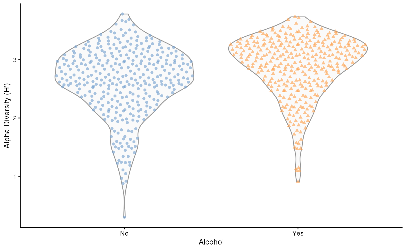
alcoholStudy |>
    estimateDiversity(assay.type = "relative_abundance", index = "shannon") |>
    plotColData(x = "alcohol", y = "shannon", colour_by = "alcohol", shape_by = "alcohol") +
    labs(x = "Alcohol", y = "Alpha Diversity (H')") +
    guides(colour = guide_legend(title = "Alcohol"), shape = guide_legend(title = "Alcohol")) +
    theme(legend.position = "none")
## Warning in estimateDiversity(alcoholStudy, assay.type = "relative_abundance", :
## 'estimateDiversity' is deprecated. Use 'addAlpha' instead.
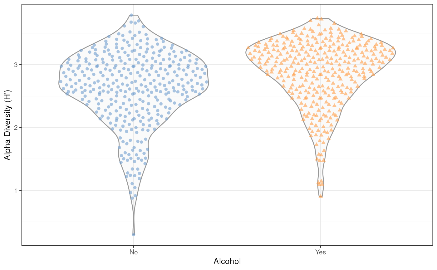
Alpha Diversity – Shannon Index (H’)
The figure suggest that those who consume alcohol have higher Shannon alpha diversity than those who do not consume alcohol; however, the difference does not appear to be significant, at least qualitatively.
Beta Diversity
Beta diversity is a measure of the between sample diversity of features (relative abundance proportions here) and seeks to quantify the magnitude of differences (or similarity) between every given pair of samples. Below it is assessed by Bray–Curtis Principal Coordinates Analysis (PCoA) and Uniform Manifold Approximation and Projection (UMAP).
Bray–Curtis PCoA
To calculate pairwise Bray–Curtis distance for every sample in our
study we will use the runMDS() function from the scater
package along with the vegdist() function from the vegan
package.
To quickly plot the results of beta diversity analysis, the
plotReducedDim() function from the scater
package is used along with ggplot2
syntax.
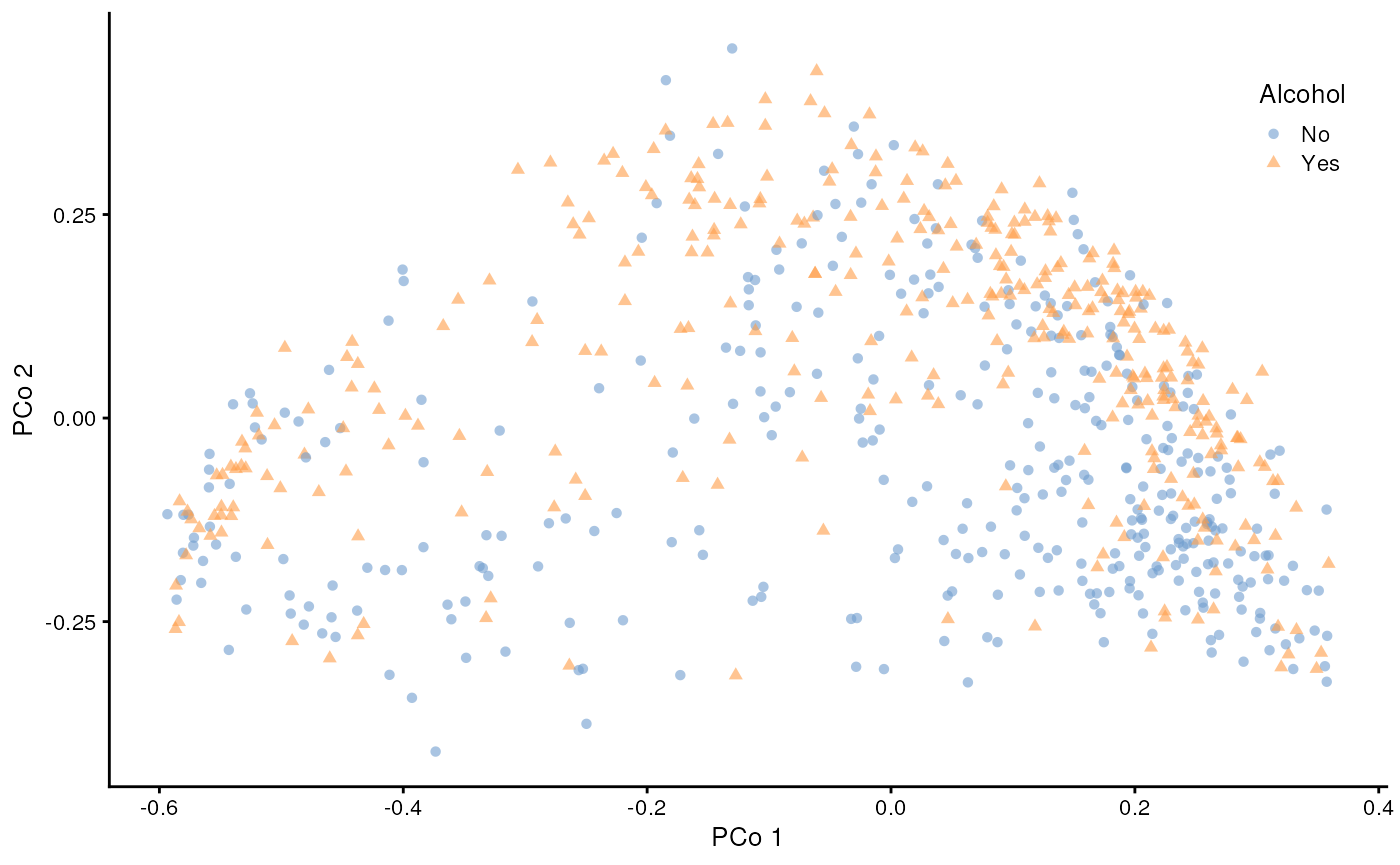
alcoholStudy |>
    runMDS(FUN = vegdist, method = "bray", exprs_values = "relative_abundance", altexp = "genus", name = "BrayCurtis") |>
    plotReducedDim("BrayCurtis", colour_by = "alcohol", shape_by = "alcohol") +
    labs(x = "PCo 1", y = "PCo 2") +
    guides(colour = guide_legend(title = "Alcohol"), shape = guide_legend(title = "Alcohol")) +
    theme(legend.position = c(0.90, 0.85))
## Warning: A numeric `legend.position` argument in `theme()` was deprecated in ggplot2
## 3.5.0.
## ℹ Please use the `legend.position.inside` argument of `theme()` instead.
## This warning is displayed once every 8 hours.
## Call `lifecycle::last_lifecycle_warnings()` to see where this warning was
## generated.
Beta Diversity – Bray–Curtis PCoA
UMAP
To calculate the UMAP coordinates of every sample in our study we
will use the runUMAP() function from the scater
package package, as it handles the task in a single line.
To quickly plot the results of beta diversity analysis, the
plotReducedDim() function from the scater
package is used along with ggplot2
syntax again.
alcoholStudy |>
    runUMAP(exprs_values = "relative_abundance", altexp = "genus", name = "UMAP") |>
    plotReducedDim("UMAP", colour_by = "alcohol", shape_by = "alcohol") +
    labs(x = "UMAP 1", y = "UMAP 2") +
    guides(colour = guide_legend(title = "Alcohol"), shape = guide_legend(title = "Alcohol")) +
    theme(legend.position = c(0.90, 0.85))
Beta Diversity – UMAP (Uniform Manifold Approximation and Projection)
Differential Abundance
Next, it would be desirable to establish which microbes are
differentially abundant between the two groups (those who consume
alcohol, and those who do not). The lefser and
ANCOMBC
packages are excellent resources for this tasks; however, code is not
included here to avoid including excessive Suggests
packages – curatedMetagenomicData
had far too many of these in the the past and is now very lean. There is
a repository of analyses, curatedMetagenomicAnalyses,
on GitHub and a forthcoming paper that will feature extensive
demonstrations of analyses – but for now, the suggestions above will
have to suffice.
Type Conversion
Finally, the curatedMetagenomicData
package previously had functions for conversion to phyloseq
class objects, and they have been removed. It is likely that some users
will still want to do analysis using phyloseq,
and we would like to help them do so – it is just easier if we don’t
have to maintain the conversion function ourselves. As such, the mia package
has a function, makePhyloseqFromTreeSummarizedExperiment,
that will readily do the conversion – users needing this functionality
are advised to use it.
convertToPhyloseq(alcoholStudy, assay.type = "relative_abundance")Session Info
## R version 4.5.0 (2025-04-11)
## Platform: x86_64-pc-linux-gnu
## Running under: Ubuntu 24.04.2 LTS
##
## Matrix products: default
## BLAS:   /usr/lib/x86_64-linux-gnu/openblas-pthread/libblas.so.3
## LAPACK: /usr/lib/x86_64-linux-gnu/openblas-pthread/libopenblasp-r0.3.26.so;  LAPACK version 3.12.0
##
## locale:
##  [1] LC_CTYPE=en_US.UTF-8       LC_NUMERIC=C
##  [3] LC_TIME=en_US.UTF-8        LC_COLLATE=en_US.UTF-8
##  [5] LC_MONETARY=en_US.UTF-8    LC_MESSAGES=en_US.UTF-8
##  [7] LC_PAPER=en_US.UTF-8       LC_NAME=C
##  [9] LC_ADDRESS=C               LC_TELEPHONE=C
## [11] LC_MEASUREMENT=en_US.UTF-8 LC_IDENTIFICATION=C
##
## time zone: Etc/UTC
## tzcode source: system (glibc)
##
## attached base packages:
## [1] stats4    stats     graphics  grDevices utils     datasets  methods
## [8] base
##
## other attached packages:
##  [1] vegan_2.6-10                    lattice_0.22-7
##  [3] permute_0.9-7                   scater_1.36.0
##  [5] ggplot2_3.5.2                   scuttle_1.18.0
##  [7] mia_1.16.0                      MultiAssayExperiment_1.34.0
##  [9] stringr_1.5.1                   DT_0.33
## [11] dplyr_1.1.4                     curatedMetagenomicData_3.16.1
## [13] TreeSummarizedExperiment_2.16.0 Biostrings_2.76.0
## [15] XVector_0.48.0                  SingleCellExperiment_1.30.0
## [17] SummarizedExperiment_1.38.0     Biobase_2.68.0
## [19] GenomicRanges_1.60.0            GenomeInfoDb_1.44.0
## [21] IRanges_2.42.0                  S4Vectors_0.46.0
## [23] BiocGenerics_0.54.0             generics_0.1.3
## [25] MatrixGenerics_1.20.0           matrixStats_1.5.0
## [27] BiocStyle_2.36.0
##
## loaded via a namespace (and not attached):
##   [1] jsonlite_2.0.0              magrittr_2.0.3
##   [3] estimability_1.5.1          ggbeeswarm_0.7.2
##   [5] farver_2.1.2                rmarkdown_2.29
##   [7] fs_1.6.6                    ragg_1.4.0
##   [9] vctrs_0.6.5                 memoise_2.0.1
##  [11] DelayedMatrixStats_1.30.0   htmltools_0.5.8.1
##  [13] S4Arrays_1.8.0              BiocBaseUtils_1.10.0
##  [15] AnnotationHub_3.16.0        curl_6.2.2
##  [17] BiocNeighbors_2.2.0         cellranger_1.1.0
##  [19] SparseArray_1.8.0           parallelly_1.43.0
##  [21] sass_0.4.10                 bslib_0.9.0
##  [23] htmlwidgets_1.6.4           desc_1.4.3
##  [25] plyr_1.8.9                  DECIPHER_3.4.0
##  [27] emmeans_1.11.0              cachem_1.1.0
##  [29] igraph_2.1.4                mime_0.13
##  [31] lifecycle_1.0.4             pkgconfig_2.0.3
##  [33] rsvd_1.0.5                  Matrix_1.7-3
##  [35] R6_2.6.1                    fastmap_1.2.0
##  [37] GenomeInfoDbData_1.2.14     digest_0.6.37
##  [39] ggnewscale_0.5.1            colorspace_2.1-1
##  [41] patchwork_1.3.0             AnnotationDbi_1.70.0
##  [43] irlba_2.3.5.1               ExperimentHub_2.16.0
##  [45] crosstalk_1.2.1             textshaping_1.0.0
##  [47] RSQLite_2.3.9               beachmat_2.24.0
##  [49] labeling_0.4.3              filelock_1.0.3
##  [51] mgcv_1.9-3                  httr_1.4.7
##  [53] abind_1.4-8                 compiler_4.5.0
##  [55] withr_3.0.2                 bit64_4.6.0-1
##  [57] BiocParallel_1.42.0         viridis_0.6.5
##  [59] DBI_1.2.3                   MASS_7.3-65
##  [61] rappdirs_0.3.3              DelayedArray_0.34.1
##  [63] bluster_1.18.0              tools_4.5.0
##  [65] vipor_0.4.7                 beeswarm_0.4.0
##  [67] ape_5.8-1                   glue_1.8.0
##  [69] nlme_3.1-168                gridtext_0.1.5
##  [71] grid_4.5.0                  cluster_2.1.8.1
##  [73] reshape2_1.4.4              gtable_0.3.6
##  [75] tzdb_0.5.0                  fillpattern_1.0.2
##  [77] tidyr_1.3.1                 hms_1.1.3
##  [79] xml2_1.3.8                  BiocSingular_1.24.0
##  [81] ScaledMatrix_1.16.0         ggrepel_0.9.6
##  [83] BiocVersion_3.21.1          pillar_1.10.2
##  [85] yulab.utils_0.2.0           splines_4.5.0
##  [87] ggtext_0.1.2                BiocFileCache_2.16.0
##  [89] treeio_1.32.0               FNN_1.1.4.1
##  [91] bit_4.6.0                   tidyselect_1.2.1
##  [93] DirichletMultinomial_1.50.0 knitr_1.50
##  [95] gridExtra_2.3               bookdown_0.43
##  [97] xfun_0.52                   rbiom_2.2.0
##  [99] stringi_1.8.7               UCSC.utils_1.4.0
## [101] lazyeval_0.2.2              yaml_2.3.10
## [103] evaluate_1.0.3              codetools_0.2-20
## [105] tibble_3.2.1                BiocManager_1.30.25
## [107] cli_3.6.4                   uwot_0.2.3
## [109] xtable_1.8-4                systemfonts_1.2.2
## [111] munsell_0.5.1               jquerylib_0.1.4
## [113] readxl_1.4.5                Rcpp_1.0.14
## [115] dbplyr_2.5.0                png_0.1-8
## [117] parallel_4.5.0              readr_2.1.5
## [119] pkgdown_2.1.1               blob_1.2.4
## [121] sparseMatrixStats_1.20.0    slam_0.1-55
## [123] mvtnorm_1.3-3               decontam_1.28.0
## [125] viridisLite_0.4.2           tidytree_0.4.6
## [127] scales_1.3.0                purrr_1.0.4
## [129] crayon_1.5.3                rlang_1.1.6
## [131] KEGGREST_1.48.0