curatedOvarianData: Clinically Annotated Data for the Ovarian Cancer Transcriptome

Benjamin Frederick Ganzfried, Markus Riester, Benjamin Haibe-Kains, Thomas Risch, Svitlana Tyekucheva, Ina Jazic, Victoria Xin Wang, Mahnaz Ahmadifar, Michael Birrer, Giovanni Parmigiani, Curtis Huttenhower, Levi Waldron

5 May 2025

Introduction

This package represents a manually curated data collection for gene expression meta-analysis of patients with ovarian cancer. This resource provides uniformly prepared microarray data with curated and documented clinical metadata. It allows a computational user to efficiently identify studies and patient subgroups of interest for analysis and to run such analyses immediately without the challenges posed by harmonizing heterogeneous microarray technologies, study designs, expression data processing methods, and clinical data formats.

The curatedOvarianData package is published in the journal DATABASE (Ganzfried et al. (2013)). Note the existence also of curatedCRCData and curatedBladderData.

Please see http://bcb.dfci.harvard.edu/ovariancancer for alterative versions of this package, differing in how redundant probe sets are dealt with.

In this vignette, we give a short tour of the package and will show how to use it efficiently.

Load TCGA data

Loading a single dataset is very easy. First we load the package:

library(curatedOvarianData)
library(sva)
library(logging)

To get a listing of all the datasets, use the data function:

data(package="curatedOvarianData")

Now to load the TCGA data, we use the data function again:

data(TCGA_eset)
TCGA_eset

## ExpressionSet (storageMode: lockedEnvironment)
## assayData: 13104 features, 578 samples 
##   element names: exprs 
## protocolData: none
## phenoData
##   sampleNames: TCGA.20.0987 TCGA.23.1031 ... TCGA.13.1819 (578 total)
##   varLabels: alt_sample_name unique_patient_ID ...
##     uncurated_author_metadata (31 total)
##   varMetadata: labelDescription
## featureData
##   featureNames: A1CF A2M ... ZZZ3 (13104 total)
##   fvarLabels: probeset gene
##   fvarMetadata: labelDescription
## experimentData: use 'experimentData(object)'
##   pubMedIds: 21720365 
## Annotation: hthgu133a

The datasets are provided as Bioconductor ExpressionSet objects and we refer to the Bioconductor documentation for users unfamiliar with this data structure.

Load datasets based on rules

For a meta-analysis, we typically want to filter datasets and patients to get a population of patients we are interested in. We provide a short but powerful R script that does the filtering and provides the data as a list of ExpressionSet objects. One can use this script within R by first sourcing a configuration file which specifies the filters, like the minimum numbers of patients in each dataset. It is also possible to filter samples by annotation, for example to remove early stage and normal samples.

source(system.file("extdata",
"patientselection.config",package="curatedOvarianData"))
ls()

##  [1] "add.surv.y"                 "duplicates"                
##  [3] "impute.missing"             "keep.common.only"          
##  [5] "meta.required"              "min.number.of.events"      
##  [7] "min.number.of.genes"        "min.sample.size"           
##  [9] "probes.not.mapped.uniquely" "quantile.cutoff"           
## [11] "remove.retracted"           "remove.samples"            
## [13] "remove.subsets"             "rescale"                   
## [15] "rule.1"                     "strict.checking"           
## [17] "TCGA_eset"                  "tcga.lowcor.outliers"

See what the values of these variables we have loaded are. The variable names are fairly descriptive, but note that “rule.1” is a character vector of length 2, where the first entry is the name of a clinical data variable, and the second entry is a Regular Expression providing a requirement for that variable. Any number of rules can be added, with increasing identifiers, e.g. “rule.2”, “rule.3”, etc.

Here strict.checking is FALSE, meaning that samples not annotated for the variables in these rules are allowed to pass the filter. If strict.checking == TRUE, samples missing this annotation will be removed.

Cleaning of duplicate samples

The patientselection.config file loaded above contains several objects indicating which samples were removed for QC and duplicate cleaning by Waldron et al. (2014) :

• tcga.lowcor.outliers: two profiles identified in the TCGA dataset with anomolously low correlation to other ovc profiles
• duplicates: samples blacklisted because they contain duplicates. In the case of duplicates, generally better-annotated samples, and samples from more recent studies, were kept.
• remove.samples: the above to vectors of samples concatenated

#remove.samples and duplicates are too voluminous:
sapply(
    ls(),
    function(x) if(!x %in% c("remove.samples", "duplicates")) print(get(x))
)

## function (X) 
## Surv(X$days_to_death, X$vital_status == "deceased")
## [1] FALSE
## [1] FALSE
## [1] "days_to_death" "vital_status" 
## [1] 15
## [1] 1000
## [1] 40
## [1] "drop"
## [1] 0
## [1] FALSE
## [1] TRUE
## [1] TRUE
## [1] "sample_type" "^tumor$"    
## [1] FALSE
## ExpressionSet (storageMode: lockedEnvironment)
## assayData: 13104 features, 578 samples 
##   element names: exprs 
## protocolData: none
## phenoData
##   sampleNames: TCGA.20.0987 TCGA.23.1031 ... TCGA.13.1819 (578 total)
##   varLabels: alt_sample_name unique_patient_ID ...
##     uncurated_author_metadata (31 total)
##   varMetadata: labelDescription
## featureData
##   featureNames: A1CF A2M ... ZZZ3 (13104 total)
##   fvarLabels: probeset gene
##   fvarMetadata: labelDescription
## experimentData: use 'experimentData(object)'
##   pubMedIds: 21720365 
## Annotation: hthgu133a 
## [1] "TCGA_eset:TCGA.24.1927" "TCGA_eset:TCGA.31.1955"

## $add.surv.y
## function (X) 
## Surv(X$days_to_death, X$vital_status == "deceased")
## 
## $duplicates
## NULL
## 
## $impute.missing
## [1] FALSE
## 
## $keep.common.only
## [1] FALSE
## 
## $meta.required
## [1] "days_to_death" "vital_status" 
## 
## $min.number.of.events
## [1] 15
## 
## $min.number.of.genes
## [1] 1000
## 
## $min.sample.size
## [1] 40
## 
## $probes.not.mapped.uniquely
## [1] "drop"
## 
## $quantile.cutoff
## [1] 0
## 
## $remove.retracted
## [1] FALSE
## 
## $remove.samples
## NULL
## 
## $remove.subsets
## [1] TRUE
## 
## $rescale
## [1] TRUE
## 
## $rule.1
## [1] "sample_type" "^tumor$"    
## 
## $strict.checking
## [1] FALSE
## 
## $TCGA_eset
## ExpressionSet (storageMode: lockedEnvironment)
## assayData: 13104 features, 578 samples 
##   element names: exprs 
## protocolData: none
## phenoData
##   sampleNames: TCGA.20.0987 TCGA.23.1031 ... TCGA.13.1819 (578 total)
##   varLabels: alt_sample_name unique_patient_ID ...
##     uncurated_author_metadata (31 total)
##   varMetadata: labelDescription
## featureData
##   featureNames: A1CF A2M ... ZZZ3 (13104 total)
##   fvarLabels: probeset gene
##   fvarMetadata: labelDescription
## experimentData: use 'experimentData(object)'
##   pubMedIds: 21720365 
## Annotation: hthgu133a 
## 
## $tcga.lowcor.outliers
## [1] "TCGA_eset:TCGA.24.1927" "TCGA_eset:TCGA.31.1955"

Now that we have defined the sample filter, we create a list of ExpressionSet objects by sourcing the createEsetList.R file:

source(system.file("extdata", "createEsetList.R", package =
"curatedOvarianData"))

## 2025-05-05 20:35:53.427904 INFO::Inside script createEsetList.R - inputArgs =
## 2025-05-05 20:35:53.45026 INFO::Loading curatedOvarianData 1.46.2
## 2025-05-05 20:36:24.285948 INFO::Clean up the esets.
## 2025-05-05 20:36:24.890901 INFO::including E.MTAB.386_eset
## 2025-05-05 20:36:24.996793 INFO::excluding GSE12418_eset (min.number.of.events or min.sample.size)
## 2025-05-05 20:36:25.156217 INFO::excluding GSE12470_eset (min.number.of.events or min.sample.size)
## 2025-05-05 20:36:25.709958 INFO::including GSE13876_eset
## 2025-05-05 20:36:25.824943 INFO::including GSE14764_eset
## 2025-05-05 20:36:26.029716 INFO::including GSE17260_eset
## 2025-05-05 20:36:26.154202 INFO::including GSE18520_eset
## 2025-05-05 20:36:26.300622 INFO::excluding GSE19829.GPL570_eset (min.number.of.events or min.sample.size)
## 2025-05-05 20:36:26.355619 INFO::including GSE19829.GPL8300_eset
## 2025-05-05 20:36:26.588578 INFO::excluding GSE20565_eset (min.number.of.events or min.sample.size)
## 2025-05-05 20:36:27.204577 INFO::excluding GSE2109_eset (min.number.of.events or min.sample.size)
## 2025-05-05 20:36:27.3725 INFO::including GSE26193_eset
## 2025-05-05 20:36:27.596635 INFO::including GSE26712_eset
## 2025-05-05 20:36:27.609935 INFO::excluding GSE30009_eset (min.number.of.genes)
## 2025-05-05 20:36:27.729004 INFO::including GSE30161_eset
## 2025-05-05 20:36:28.089588 INFO::including GSE32062.GPL6480_eset
## 2025-05-05 20:36:28.215789 INFO::excluding GSE32063_eset (min.number.of.events or min.sample.size)
## 2025-05-05 20:36:28.333604 INFO::excluding GSE44104_eset (min.number.of.events or min.sample.size)
## 2025-05-05 20:36:28.601136 INFO::including GSE49997_eset
## 2025-05-05 20:36:29.060841 INFO::including GSE51088_eset
## 2025-05-05 20:36:29.161267 INFO::excluding GSE6008_eset (min.number.of.events or min.sample.size)
## 2025-05-05 20:36:29.202401 INFO::excluding GSE6822_eset (min.number.of.events or min.sample.size)
## 2025-05-05 20:36:29.254688 INFO::excluding GSE8842_eset (min.number.of.events or min.sample.size)
## 2025-05-05 20:36:29.97657 INFO::including GSE9891_eset
## 2025-05-05 20:36:30.059227 INFO::excluding PMID15897565_eset (min.number.of.events or min.sample.size)
## 2025-05-05 20:36:30.178745 INFO::including PMID17290060_eset
## 2025-05-05 20:36:30.283902 INFO::excluding PMID19318476_eset (min.number.of.events or min.sample.size)
## 2025-05-05 20:36:30.711557 INFO::including TCGA_eset
## 2025-05-05 20:36:30.743423 INFO::excluding TCGA.mirna.8x15kv2_eset (min.number.of.genes)
## 2025-05-05 20:36:31.458084 INFO::including TCGA.RNASeqV2_eset
## 2025-05-05 20:36:31.85711 INFO::Ids with missing data: GSE51088_eset, TCGA.RNASeqV2_eset

It is also possible to run the script from the command line and then load the R data file within R:

R --vanilla "--args patientselection.config ovarian.eset.rda tmp.log"  < createEsetList.R

Now we have datasets with samples that passed our filter in a list of ExpressionSet objects called esets:

names(esets)

##  [1] "E.MTAB.386_eset"       "GSE13876_eset"         "GSE14764_eset"        
##  [4] "GSE17260_eset"         "GSE18520_eset"         "GSE19829.GPL8300_eset"
##  [7] "GSE26193_eset"         "GSE26712_eset"         "GSE30161_eset"        
## [10] "GSE32062.GPL6480_eset" "GSE49997_eset"         "GSE51088_eset"        
## [13] "GSE9891_eset"          "PMID17290060_eset"     "TCGA_eset"            
## [16] "TCGA.RNASeqV2_eset"

Association of CXCL12 expression with overall survival

Next we use the list of datasets from the previous example and test if the expression of the CXCL12 gene is associated with overall survival. CXCL12/CXCR4 is a chemokine/chemokine receptor axis that has previously been shown to be directly involved in cancer pathogenesis.

We first define a function that will generate a forest plot for a given gene. It needs the overall survival information as Surv objects, which the createEsetList.R function already added in the phenoData slots of the ExpressionSet objects, accessible at the y label. The resulting forest plot is shown for the CXCL12 gene in the figure below.

esets[[1]]$y

##   [1]  840.9+  399.9+  524.1+ 1476.0   144.0   516.9   405.0    87.0    45.9+
##  [10]  483.9+  917.1  1013.1+   69.9   486.0   369.9  2585.1+  738.9   362.1 
##  [19] 2031.9+  477.9  1091.1+ 1062.0+  720.9  1200.9+  977.1   537.9   638.1 
##  [28]  587.1  1509.0  1619.1+ 1043.1   198.9  1520.1   696.9  1140.9  1862.1+
##  [37] 1751.1+ 1845.0+ 1197.0  1401.0   399.0   992.1   927.9+ 1509.0  1914.0+
##  [46]  591.9   426.0  1374.9+  546.9   809.1+  480.9+  486.0+  642.9+  540.9+
##  [55]  962.1  2025.0   473.1  1140.0   512.1  1002.9+ 1731.9+  690.0   930.0 
##  [64] 1026.9  1193.1+  720.9   369.0  1326.9+  501.9+ 1677.0+ 1773.9+  251.1 
##  [73] 1338.9+   35.1  1467.9+  165.9   981.9  1280.1  1800.0+  399.9   422.1 
##  [82]  861.9  2010.0+  660.0  2138.1+  516.0+ 1001.1+  693.9   825.0+  815.1+
##  [91]  657.0+ 1013.1+  426.0   656.1  1356.0  1610.1+ 1068.9+ 1221.9+ 2388.0+
## [100]  447.9+  602.1+ 1875.0+  920.1+  959.1   708.0   546.0  1254.9+  611.1+
## [109] 1317.9  1899.0  1886.1   642.0  1763.1  1857.0+  540.0   852.9   498.0+
## [118]    3.9+  836.1  1452.0  2721.0   450.9  1398.9  1481.1  2724.0+ 2061.9 
## [127]  651.9  2349.0+

forestplot <- function(esets, y="y", probeset, formula=y~probeset,
mlab="Overall", rma.method="FE", at=NULL,xlab="Hazard Ratio",...) {
    require(metafor)
    esets <- esets[sapply(esets, function(x) probeset %in% featureNames(x))]
    coefs <- sapply(1:length(esets), function(i) {
        tmp   <- as(phenoData(esets[[i]]), "data.frame")
        tmp$y <- esets[[i]][[y]]
        tmp$probeset <- exprs(esets[[i]])[probeset,]

        summary(coxph(formula,data=tmp))$coefficients[1,c(1,3)]
    })

    res.rma <- metafor::rma(yi = coefs[1,], sei = coefs[2,],
        method=rma.method)

    if (is.null(at)) at <- log(c(0.25,1,4,20))
    forest.rma(res.rma, xlab=xlab, slab=gsub("_eset$","",names(esets)),
    atransf=exp, at=at, mlab=mlab,...)
    return(res.rma)
}

res <- forestplot(esets=esets,probeset="CXCL12",at=log(c(0.5,1,2,4)))

## Loading required package: metafor

## Loading required package: Matrix

## Loading required package: metadat

## Loading required package: numDeriv

## 
## Loading the 'metafor' package (version 4.8-0). For an
## introduction to the package please type: help(metafor)

Figure 1: The database confirms CXCL12 as prognostic of overall survival in patients with ovarian cancer. Forest plot of the expression of the chemokine CXCL12 as a univariate predictor of overall survival, using all datasets with applicable expression and survival information. A hazard ratio significantly larger than 1 indicates that patients with high CXCL12 levels had poor outcome. The p-value for the overall HR, found in res$pval, is 9^{-10}. This plot is Figure 3 of the curatedOvarianData manuscript.

We now test whether CXCL12 is an independent predictor of survival in a multivariate model together with success of debulking surgery, defined as residual tumor smaller than 1 cm, and Federation of Gynecology and Obstetrics (FIGO) stage. We first filter the datasets without debulking and stage information:

idx.tumorstage <- sapply(esets, function(X)
    sum(!is.na(X$tumorstage)) > 0 & length(unique(X$tumorstage)) > 1)

idx.debulking <- sapply(esets, function(X)
    sum(X$debulking=="suboptimal",na.rm=TRUE)) > 0

In the figure below, we see that CXCL12 stays significant after adjusting for debulking status and FIGO stage. We repeated this analysis for the CXCR4 receptor and found no significant association with overall survival (Figure 3).

res <- forestplot(esets=esets[idx.debulking & idx.tumorstage],
    probeset="CXCL12",formula=y~probeset+debulking+tumorstage,
    at=log(c(0.5,1,2,4)))

Figure 2: Validation of CXCL12 as an independent predictor of survival. This figure shows a forest plot as in Figure 1, but the CXCL12 expression levels were adjusted for debulking status (optimal versus suboptimal) and tumor stage. The p-value for the overall HR, found in res$pval, is `r signif(res$pval, 2)`.

res <- forestplot(esets=esets,probeset="CXCR4",at=log(c(0.5,1,2,4)))

Figure 3: Up-regulation of CXCR4 is not associated with overall survival. This figure shows again a forest plot as in Figure 1, but here the association of mRNA expression levels of the CXCR4 receptor and overall survival is shown. The p-value for the overall HR, found in res$pval, is 0.12.

Batch correction with ComBat

If datasets are merged, it is typically recommended to remove a very likely batch effect. We will use the ComBat (Johnson, Li, and Rabinovic 2007) method, implemented for example in the SVA Bioconductor package (Leek et al., n.d.). To combine two ExpressionSet objects, we can use the combine() function. This function will fail when the two ExpressionSets have conflicting annotation slots, for example annotation when the platforms differ. We write a simple combine2 function which only considers the exprs and phenoData slots:

combine2 <- function(X1, X2) {
    fids <- intersect(featureNames(X1), featureNames(X2))
    X1 <- X1[fids,]
    X2 <- X2[fids,]
    ExpressionSet(cbind(exprs(X1),exprs(X2)),
        AnnotatedDataFrame(rbind(as(phenoData(X1),"data.frame"),
                                 as(phenoData(X2),"data.frame")))
    )
}

In Figure 4, we combined two datasets from different platforms, resulting in a huge batch effect.

data(E.MTAB.386_eset)
data(GSE30161_eset)
X <- combine2(E.MTAB.386_eset, GSE30161_eset)
boxplot(exprs(X))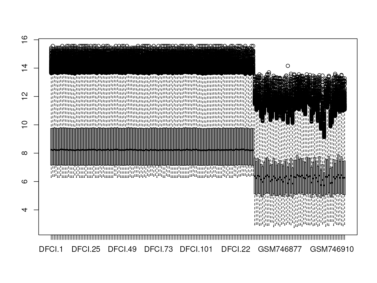

Figure 4: Boxplot showing the expression range for all samples of two merged datasets arrayed on different platforms. This illustrates a huge batch effect.

Now we apply ComBat and adjust for the batch and show the boxplot after batch correction in Figure 5:

mod <- model.matrix(~as.factor(tumorstage), data=X)
batch <- as.factor(grepl("DFCI",sampleNames(X)))
combat_edata <- ComBat(dat=exprs(X), batch=batch, mod=mod)

## Found2batches

## Adjusting for2covariate(s) or covariate level(s)

## Standardizing Data across genes

## Fitting L/S model and finding priors

## Finding parametric adjustments

## Adjusting the Data

boxplot(combat_edata)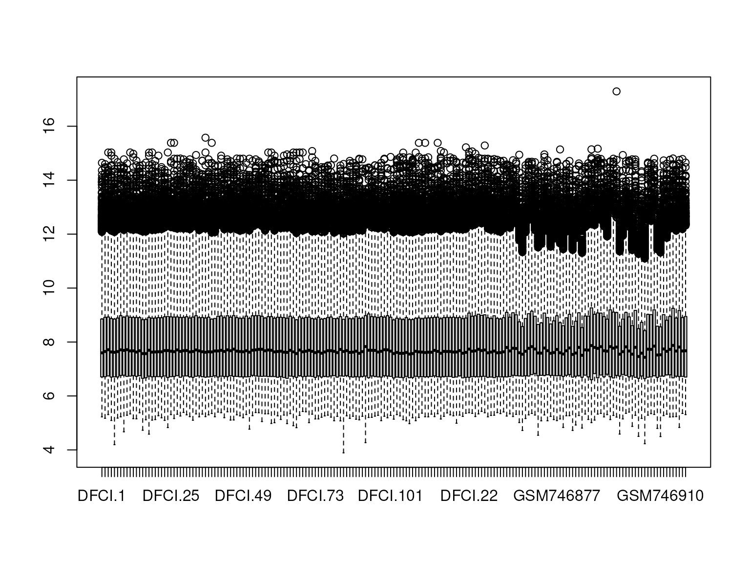

Figure 5: Boxplot showing the expression range for all samples of two merged datasets arrayed on different platforms after batch correction with ComBat.

Non-specific probe sets

In the standard version of curatedOvarianData (the version available on Bioconductor), we collapse manufacturer probesets to official HGNC symbols using the Biomart database. Some probesets are mapped to multiple HGNC symbols in this database. For these probesets, we provide all the symbols. For example 220159_at maps to ABCA11P and ZNF721 and we provide ABCA11P///ZNF721 as probeset name. If you have an array of gene symbols for which you want to access the expression data, “ABCA11P” would not be found in curatedOvarianData in this example.

The script createEsetList.R provides three methods to deal with non-specific probe sets by setting the variable $probes.not.mapped.uniquely$ to:

• “keep”: leave as-is, these have “///” in gene names,
• “drop”: drop any non-uniquely mapped features, or
• “split”: split non-uniquely mapped features to one per row. If this creates duplicate rows for a gene, those rows are averaged.

This feature uses the following function to create a new ExpressionSet, in which both ZNF721 and ABCA11P are features with identical expression data:

expandProbesets <- function (eset, sep = "///")
{
    x <- lapply(featureNames(eset), function(x) strsplit(x, sep)[[1]])
    eset <- eset[order(sapply(x, length)), ]
    x <- lapply(featureNames(eset), function(x) strsplit(x, sep)[[1]])
    idx <- unlist(sapply(1:length(x), function(i) rep(i, length(x[[i]]))))
    xx <- !duplicated(unlist(x))
    idx <- idx[xx]
    x <- unlist(x)[xx]
    eset <- eset[idx, ]
    featureNames(eset) <- x
    eset
}

X <- TCGA_eset[head(grep("///", featureNames(TCGA_eset))),]
exprs(X)[,1:3]

##                                                         TCGA.20.0987
## ABCB4///ABCB1                                               2.993923
## ABCB6///ATG9A                                               4.257024
## ABCC6P2///ABCC6P1///ABCC6                                   3.110547
## ABHD17AP3///ABHD17AP2///ABHD17AP1///ABHD17AP6///ABHD17A     6.886997
## ACOT1///ACOT2                                               4.702057
## ACSM2A///ACSM2B                                             2.980667
##                                                         TCGA.23.1031
## ABCB4///ABCB1                                               3.600534
## ABCB6///ATG9A                                               4.793526
## ABCC6P2///ABCC6P1///ABCC6                                   4.909549
## ABHD17AP3///ABHD17AP2///ABHD17AP1///ABHD17AP6///ABHD17A     6.699198
## ACOT1///ACOT2                                               3.534889
## ACSM2A///ACSM2B                                             3.085545
##                                                         TCGA.24.0979
## ABCB4///ABCB1                                               3.539278
## ABCB6///ATG9A                                               5.476369
## ABCC6P2///ABCC6P1///ABCC6                                   4.993433
## ABHD17AP3///ABHD17AP2///ABHD17AP1///ABHD17AP6///ABHD17A     6.529303
## ACOT1///ACOT2                                               3.604559
## ACSM2A///ACSM2B                                             2.890781

exprs(expandProbesets(X))[,1:3]

##           TCGA.20.0987 TCGA.23.1031 TCGA.24.0979
## ABCB4         2.993923     3.600534     3.539278
## ABCB1         2.993923     3.600534     3.539278
## ABCB6         4.257024     4.793526     5.476369
## ATG9A         4.257024     4.793526     5.476369
## ACOT1         4.702057     3.534889     3.604559
## ACOT2         4.702057     3.534889     3.604559
## ACSM2A        2.980667     3.085545     2.890781
## ACSM2B        2.980667     3.085545     2.890781
## ABCC6P2       3.110547     4.909549     4.993433
## ABCC6P1       3.110547     4.909549     4.993433
## ABCC6         3.110547     4.909549     4.993433
## ABHD17AP3     6.886997     6.699198     6.529303
## ABHD17AP2     6.886997     6.699198     6.529303
## ABHD17AP1     6.886997     6.699198     6.529303
## ABHD17AP6     6.886997     6.699198     6.529303
## ABHD17A       6.886997     6.699198     6.529303

FULLVcuratedOvarianData

In curatedOvarianData, probesets mapping to the same gene symbol are merge by selecting the probeset with maximum mean across all studies of a given platform. You can see which representative probeset was chosen by looking at the featureData of the Expressionset, e.g.:

head(pData(featureData(GSE18520_eset)))

##             probeset     gene
## A1BG       229819_at     A1BG
## A1BG-AS1 232462_s_at A1BG-AS1
## A1CF     220951_s_at     A1CF
## A2M        217757_at      A2M
## A2M-AS1   1564139_at  A2M-AS1
## A2ML1     1553505_at    A2ML1

The full, unmerged ExpressionSets are available through the FULLVcuratedOvarianData package at http://bcb.dfci.harvard.edu/ovariancancer/. Probeset to gene maps are again provided in the featureData of those ExpressionSets. Where official Bioconductor annotation packages are available for the array, these are stored in the ExpressionSet annotation slots, e.g.:

annotation(GSE18520_eset)

## [1] "hgu133plus2"

so that standard filtering methods such as nsFilter will work by default.

Available Clinical Characteristics

Figure 6: Available clinical annotation. This heatmap visualizes for each curated clinical characteristic (rows) the availability in each dataset (columns). Red indicates that the corresponding characteristic is available for at least one sample in the dataset. This plot is Figure 2 of the curatedOvarianData manuscript.

Summarizing the List of ExpressionSets

This example provides a table summarizing the datasets being used, and is useful when publishing analyses based on curatedOvarianData. First, define some useful functions for this purpose:

source(system.file("extdata", "summarizeEsets.R", package =
    "curatedOvarianData"))

Now create the table, used for Table 1 of the curatedOvarianData manuscript:

## Warning in min(which(km.fit$surv < 0.5)): no non-missing arguments to min;
## returning Inf
## Warning in min(which(km.fit$surv < 0.5)): no non-missing arguments to min;
## returning Inf

Optionally write this table to file, for example (replace myfile <- tempfile() with something like myfile <- “nicetable.csv”)

(myfile <- tempfile())

## [1] "/tmp/RtmpDbnirh/file173d1ceb9fb2"

write.table(summary.table, file=myfile, row.names=FALSE, quote=TRUE, sep=",")

Datasets provided by curatedOvarianData. This is an abbreviated version of Table 1 of the manuscript; the full version is written by the write.table command above. Stage column is early/late/unknown, histology column is ser/clearcell/endo/mucinous/other/unknown.

	PMID	N samples	stage	histology	Platform
E.MTAB.386	22348002	129	1/128/0	129/0/0/0/0/0/0	Illumina humanRef-8 v2.0
GSE12418	16996261	54	0/54/0	54/0/0/0/0/0/0	SWEGENE H_v2.1.1_27k
GSE12470	19486012	53	8/35/10	43/0/0/0/0/0/10	Agilent G4110B
GSE13876	19192944	157	0/157/0	157/0/0/0/0/0/0	Operon v3 two-color
GSE14764	19294737	80	9/71/0	68/2/6/0/2/0/2	Affymetrix HG-U133A
GSE17260	20300634	110	0/110/0	110/0/0/0/0/0/0	Agilent G4112A
GSE18520	19962670	63	0/53/10	53/0/0/0/0/0/10	Affymetrix HG-U133Plus2
GSE19829.GPL570	20547991	28	0/0/28	0/0/0/0/0/0/28	Affymetrix HG-U133Plus2
GSE19829.GPL8300	20547991	42	0/0/42	0/0/0/0/0/0/42	Affymetrix HG_U95Av2
GSE20565	20492709	140	27/67/46	71/6/6/7/6/0/44	Affymetrix HG-U133Plus2
GSE2109	PMID unknown	204	37/87/80	85/9/28/11/59/0/12	Affymetrix HG-U133Plus2
GSE26193	22101765	107	31/76/0	79/6/8/8/6/0/0	Affymetrix HG-U133Plus2
GSE26712	18593951	195	0/185/10	185/0/0/0/0/0/10	Affymetrix HG-U133A
GSE30009	22492981	103	0/103/0	102/1/0/0/0/0/0	TaqMan qRT-PCR
GSE30161	22348014	58	0/58/0	47/5/1/1/1/0/3	Affymetrix HG-U133Plus2
GSE32062.GPL6480	22241791	260	0/260/0	260/0/0/0/0/0/0	Agilent G4112F
GSE32063	22241791	40	0/40/0	40/0/0/0/0/0/0	Agilent G4112F
GSE44104	23934190	60	25/35/0	28/12/11/9/0/0/0	Affymetrix HG-U133Plus2
GSE49997	22497737	204	9/185/10	171/0/0/0/23/0/10	ABI Human Genome
GSE51088	24368280	172	31/120/21	122/3/7/9/11/0/20	Agilent G4110B
GSE6008	19440550	103	42/53/8	41/8/37/13/0/0/4	Affymetrix HG-U133A
GSE6822	PMID unknown	66	0/0/66	41/11/7/1/0/0/6	Affymetrix Hu6800
GSE8842	19047114	83	83/0/0	31/16/17/17/1/0/1	Agilent G4100A cDNA
GSE9891	18698038	285	42/240/3	264/0/20/0/1/0/0	Affymetrix HG-U133Plus2
PMID15897565	15897565	63	11/52/0	63/0/0/0/0/0/0	Affymetrix HG-U133A
PMID17290060	17290060	117	1/115/1	117/0/0/0/0/0/0	Affymetrix HG-U133A
PMID19318476	19318476	42	2/39/1	42/0/0/0/0/0/0	Affymetrix HG-U133A
TCGA	21720365	578	43/520/15	568/0/0/0/0/0/10	Affymetrix HT_HG-U133A
TCGA.mirna.8x15kv2	21720365	554	39/511/4	554/0/0/0/0/0/0	Agilent miRNA-8x15k2 G4470B
TCGA.RNASeqV2	21720365	261	18/242/1	261/0/0/0/0/0/0	Illumina HiSeq RNA sequencing

For non-R users

If you are not doing your analysis in R, and just want to get some data you have identified from the curatedOvarianData manual, here is a simple way to do it. For one dataset:

library(curatedOvarianData)
data(GSE30161_eset)
write.csv(exprs(GSE30161_eset), file="GSE30161_eset_exprs.csv")
write.csv(pData(GSE30161_eset), file="GSE30161_eset_clindata.csv")

Or for several datasets:

data.to.fetch <- c("GSE30161_eset", "E.MTAB.386_eset")
for (onedata in data.to.fetch){
    print(paste("Fetching", onedata))
    data(list=onedata)
    write.csv(exprs(get(onedata)), file=paste(onedata, "_exprs.csv", sep=""))
    write.csv(pData(get(onedata)), file=paste(onedata, "_clindata.csv", sep=""))
}

Session Info

sessionInfo()

## R version 4.5.0 (2025-04-11)
## Platform: x86_64-pc-linux-gnu
## Running under: Ubuntu 24.04.2 LTS
## 
## Matrix products: default
## BLAS:   /usr/lib/x86_64-linux-gnu/openblas-pthread/libblas.so.3 
## LAPACK: /usr/lib/x86_64-linux-gnu/openblas-pthread/libopenblasp-r0.3.26.so;  LAPACK version 3.12.0
## 
## locale:
##  [1] LC_CTYPE=en_US.UTF-8       LC_NUMERIC=C              
##  [3] LC_TIME=en_US.UTF-8        LC_COLLATE=en_US.UTF-8    
##  [5] LC_MONETARY=en_US.UTF-8    LC_MESSAGES=en_US.UTF-8   
##  [7] LC_PAPER=en_US.UTF-8       LC_NAME=C                 
##  [9] LC_ADDRESS=C               LC_TELEPHONE=C            
## [11] LC_MEASUREMENT=en_US.UTF-8 LC_IDENTIFICATION=C       
## 
## time zone: Etc/UTC
## tzcode source: system (glibc)
## 
## attached base packages:
## [1] stats     graphics  grDevices utils     datasets  methods   base     
## 
## other attached packages:
##  [1] metafor_4.8-0             numDeriv_2016.8-1.1      
##  [3] metadat_1.4-0             Matrix_1.7-3             
##  [5] survival_3.8-3            logging_0.10-108         
##  [7] sva_3.56.0                BiocParallel_1.42.0      
##  [9] genefilter_1.90.0         mgcv_1.9-3               
## [11] nlme_3.1-168              curatedOvarianData_1.46.2
## [13] Biobase_2.68.0            BiocGenerics_0.54.0      
## [15] generics_0.1.3            BiocStyle_2.36.0         
## 
## loaded via a namespace (and not attached):
##  [1] KEGGREST_1.48.0         xfun_0.52               bslib_0.9.0            
##  [4] htmlwidgets_1.6.4       lattice_0.22-7          mathjaxr_1.8-0         
##  [7] vctrs_0.6.5             tools_4.5.0             stats4_4.5.0           
## [10] parallel_4.5.0          AnnotationDbi_1.70.0    RSQLite_2.3.11         
## [13] blob_1.2.4              desc_1.4.3              S4Vectors_0.46.0       
## [16] lifecycle_1.0.4         GenomeInfoDbData_1.2.14 compiler_4.5.0         
## [19] textshaping_1.0.1       Biostrings_2.76.0       statmod_1.5.0          
## [22] codetools_0.2-20        GenomeInfoDb_1.44.0     htmltools_0.5.8.1      
## [25] sass_0.4.10             yaml_2.3.10             pkgdown_2.1.2          
## [28] crayon_1.5.3            jquerylib_0.1.4         cachem_1.1.0           
## [31] limma_3.64.0            locfit_1.5-9.12         digest_0.6.37          
## [34] bookdown_0.43           splines_4.5.0           fastmap_1.2.0          
## [37] grid_4.5.0              cli_3.6.5               XML_3.99-0.18          
## [40] edgeR_4.6.1             UCSC.utils_1.4.0        bit64_4.6.0-1          
## [43] rmarkdown_2.29          XVector_0.48.0          httr_1.4.7             
## [46] matrixStats_1.5.0       bit_4.6.0               ragg_1.4.0             
## [49] png_0.1-8               memoise_2.0.1           evaluate_1.0.3         
## [52] knitr_1.50              IRanges_2.42.0          rlang_1.1.6            
## [55] xtable_1.8-4            DBI_1.2.3               BiocManager_1.30.25    
## [58] annotate_1.86.0         jsonlite_2.0.0          R6_2.6.1               
## [61] MatrixGenerics_1.20.0   systemfonts_1.2.3       fs_1.6.6

References

Ganzfried, Benjamin Frederick, Markus Riester, Benjamin Haibe-Kains, Thomas Risch, Svitlana Tyekucheva, Ina Jazic, Xin Victoria Wang, et al. 2013. “curatedOvarianData: Clinically Annotated Data for the Ovarian Cancer Transcriptome.” Database 2013: bat013.

Johnson, W E, C Li, and A Rabinovic. 2007. “Adjusting Batch Effects in Microarray Expression Data Using Empirical Bayes Methods.” Biostatistics 8 (1): 118–27.

Leek, Jeffrey T., W. Evan Johnson, Hilary S. Parker, Andrew E. Jaffe, and John D. Storey. n.d. Sva: Surrogate Variable Analysis.

Waldron, Levi, Benjamin Haibe-Kains, Aedı́n C Culhane, Markus Riester, Jie Ding, Xin Victoria Wang, Mahnaz Ahmadifar, et al. 2014. “Comparative Meta-Analysis of Prognostic Gene Signatures for Late-Stage Ovarian Cancer.” J. Natl. Cancer Inst. 106 (5). https://doi.org/10.1093/jnci/dju049.