simulate correlated predictors with time-to-event or binary outcome

This function creates multiple groups of predictor variables which may be correlated within each group, and binary or survival time (without censoring) response according to specified weights of the predictors.

create.data(nvars = c(100, 100, 100, 100, 600),
            cors = c(0.8, 0, 0.8, 0, 0),
            associations = c(0.5, 0.5, 0.3, 0.3, 0),
            firstonly = c(TRUE, FALSE, TRUE, FALSE, FALSE),
            nsamples = 100,
            censoring = "none",
            labelswapprob = 0,
            response = "timetoevent",
            basehaz = 0.2,
            logisticintercept = 0)

Arguments

nvars	integer vector giving the number of variables of each variable type. The number of variable types is equal to the length of this vector.
cors	integer vector of the same length as nvars, giving the population pairwise Pearson correlation within each group.
associations	integer vector of the same length as nvars, giving the associations of each type with outcome
firstonly	logical vector of the same length as nvars, specifying whether only the first variable of each type is associated with outcome (TRUE) or all variables of that type (FALSE)
nsamples	an integer giving the number of observations
censoring	"none" for no censoring, or a vector of length two c(a,b) for uniform U(a,b) censoring.
labelswapprob	This provides an option to add uncertainty to binary outcomes by randomly switching labels with probability labelswapprob. The probability of a label being swapped is independent for each observation. The value is ignored if response is "timetoevent"
response	either "timetoevent" or "binary"
basehaz	baseline hazard, used for "timetoevent"
logisticintercept	intercept which is added to X%*%Beta for "binary"

Details

This function simulates "predictor" variables in one or more groups, which are standard normally distributed. The user can specify the population correlation within each variable group, the association of each variable group to outcome, and whether the first or all variables of that type should be associated with outcome. The simulated response variable can be time to event with an exponential distribution, or binary survival with a logistic distribution.

Value

Returns a list with items:

summary

a summary of the variable types produced

associations

weights of each variable in computing the outcome

covariance

covariance matrix used for generating potentially correlated random predictors

data

dataframe containing the predictors and response. Response is the last column for binary outcome ("outcome"), and the last two columns for timetoevent outcome ("time" and "cens")

References

Waldron L., Pintilie M., Tsao M.-S., Shepherd F. A., Huttenhower C.*, and Jurisica I.* Optimized application of penalized regression methods to diverse genomic data. (2010). Under review. (*equal contribution)

Note

Depends on the MASS package for correlated random number generation

Examples

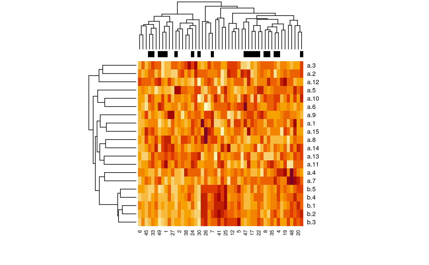
##binary outcome example
set.seed(9)
x <-
  create.data(
    nvars = c(15, 5),
    cors = c(0, 0.8),
    associations = c(0, 2),
    firstonly = c(TRUE, TRUE),
    nsamples = 50,
    response = "binary",
    logisticintercept = 0.5
  )
summary(x)
#>              Length Class      Mode   
#> summary        6    data.frame list   
#> associations  20    -none-     numeric
#> covariance   400    -none-     numeric
#> data          21    data.frame list   
x$summary
#>   start end cors associations num firstonly
#> a     1  15  0.0            0  15      TRUE
#> b    16  20  0.8            2   5      TRUE
model <- glm(outcome ~ .,  data = x$data, family = binomial)
#> Warning: glm.fit: algorithm did not converge
#> Warning: glm.fit: fitted probabilities numerically 0 or 1 occurred
summary(model)
#> 
#> Call:
#> glm(formula = outcome ~ ., family = binomial, data = x$data)
#> 
#> Deviance Residuals: 
#>        Min          1Q      Median          3Q         Max  
#> -2.156e-04  -2.100e-08   2.100e-08   4.490e-06   2.110e-04  
#> 
#> Coefficients:
#>               Estimate Std. Error z value Pr(>|z|)
#> (Intercept)    394.817  40723.092   0.010    0.992
#> a.1             -2.017   8340.192   0.000    1.000
#> a.2           1054.116 107650.687   0.010    0.992
#> a.3            432.929  41344.208   0.010    0.992
#> a.4            187.507  21631.886   0.009    0.993
#> a.5           -403.302  39003.798  -0.010    0.992
#> a.6           -236.102  20862.924  -0.011    0.991
#> a.7           -258.201  23085.549  -0.011    0.991
#> a.8              7.364  18988.262   0.000    1.000
#> a.9            229.596  21020.703   0.011    0.991
#> a.10          -519.764  55465.620  -0.009    0.993
#> a.11          -718.759  73461.234  -0.010    0.992
#> a.12            94.096  16745.928   0.006    0.996
#> a.13          -619.513  65350.574  -0.009    0.992
#> a.14           585.887  61785.544   0.009    0.992
#> a.15          -271.199  30368.663  -0.009    0.993
#> b.1            447.844  49587.944   0.009    0.993
#> b.2           -100.723  21001.800  -0.005    0.996
#> b.3           -197.254  35209.129  -0.006    0.996
#> b.4           1540.346 146783.886   0.010    0.992
#> b.5          -1080.818 105901.366  -0.010    0.992
#> 
#> (Dispersion parameter for binomial family taken to be 1)
#> 
#>     Null deviance: 6.6406e+01  on 49  degrees of freedom
#> Residual deviance: 3.7489e-07  on 29  degrees of freedom
#> AIC: 42
#> 
#> Number of Fisher Scoring iterations: 25
#> 
dat <- t(as.matrix(x$data[, -match("outcome", colnames(x$data))]))
heatmap(dat, ColSideColors = ifelse(x$data$outcome == 0, "black", "white"))

##censored survival outcome example:
set.seed(1)
x <- create.data(
  nvars = c(15, 5),
  cors = c(0, 0.8),
  associations = c(0, 2),
  firstonly = c(TRUE, TRUE),
  nsamples = 50,
  censoring = c(2, 10),
  response = "timetoevent"
)
sum(x$data$cens == 0) / nrow(x$data)  #34 percent censoring
#> [1] 0.44

library(survival)
surv.obj <- Surv(x$data$time, x$data$cens)
plot(survfit(surv.obj ~ 1), ylab = "Survival probability", xlab = "time")