Introduction
This package acts as a wrapper to the penalized R package to add the following functionality to that package:
- repeated tuning on different data folds, with parallelization to take advantage of multiple processors
- two-dimensional tuning of the Elastic Net
- calculation of cross-validated risk scores through a nested cross-validation procedure, with parallelization to take advantage of multiple processors
It also provides a function for simulation of collinear high-dimensional data with survival or binary response.
This package was developed in support of the study by Waldron et al. (2011).
This paper contains greater detail on proper application of the methods provided here. Please cite this paper when using the pensim package in your research, as well as the penalized package (Goeman (2010)).
Example data
pensim provides example data from a microarray experiment investigating survival of cancer patients with lung adenocarcinomas (Beer et al. (2002)). Load this data and do an initial pre-filter of genes with low IQR:
library(pensim)
data(beer.exprs)
data(beer.survival)
##select just 100 genes to speed computation, just for the sake of example:
set.seed(1)
beer.exprs.sample <- beer.exprs[sample(1:nrow(beer.exprs), 100),]
#
gene.quant <- apply(beer.exprs.sample, 1, quantile, probs = 0.75)
dat.filt <- beer.exprs.sample[gene.quant > log2(100),]
gene.iqr <- apply(dat.filt, 1, IQR)
dat.filt <- as.matrix(dat.filt[gene.iqr > 0.5,])
dat.filt <- t(dat.filt)
dat.filt <- data.frame(dat.filt)
#
library(survival)
surv.obj <- Surv(beer.survival$os, beer.survival$status)
Note that the expression data are in “wide” format, with one column per predictor (gene). It is recommended to put covariate data in a dataframe object, rather than a matrix.
Nested cross-validation
Unbiased estimation of prediction accuracy involves two levels of cross-validation: an outer level for estimating prediction accuracy, and an inner level for model tuning. This process is simplified by the opt.nested.crossval function.
It is recommended first to establish the arguments for the penalized regression by testing on the penalized package functions optL1 (for LASSO), optL2 (for Ridge) or cvl (for Elastic Net). Here we use LASSO. Setting maxlambda1=5 is not a generally recommended procedure, but is useful in this toy example to avoid converging on the null model.
library(penalized)
## Welcome to penalized. For extended examples, see vignette("penalized").testfit <- optL1( response = surv.obj, penalized = dat.filt, fold = 5, maxlambda1 = 5, positive = FALSE, standardize = TRUE, trace = FALSE )
Now pass these arguments to opt.nested.crossval() for cross-validated calculation and assessment of risk scores, with the additional arguments:
-
outerfoldandnprocessors: number of folds for the outer level of cross-validation, and the number of processors to use for the outer level of cross-validation (see?opt.nested.crossval) - optFUN and scaling: which optimization function to use (
opt1Dfor LASSO or Ridge,opt2Dfor Elastic Net) - see?opt.splitval. - setpen and nsim: setpen defines whether to do LASSO (“L1”) or Ridge (“L2”),
nsimdefines the number of times to repeat tuning (see?opt1D.opt2Dhas different required arguments.)
set.seed(1)
preds <-
  opt.nested.crossval(
    outerfold = 5,
    nprocessors = 1,
    #opt.nested.crossval arguments
    optFUN = "opt1D",
    scaling = FALSE,
    #opt.splitval arguments
    setpen = "L1",
    nsim = 1,
    #opt1D arguments
    response = surv.obj,
    #rest are penalized::optl1 arguments
    penalized = dat.filt,
    fold = 5,
    positive = FALSE,
    standardize = TRUE,
    trace = FALSE
  )
Ideally nsim would be 50, and outerfold and fold would be 10, but the values below speed computation 200x compared to these recommended values. Note that here we are using the standardize=TRUE argument of optL1 rather than the scaling=TRUE argument of opt.splitval. These two approaches to scaling are roughly equivalent, but the scaling approaches are not the same (scaling=TRUE does z-score, standardize=TRUE scales to unit central L2 norm), and results will not be identical. Also, using standardize=TRUE scales variables but provides coeffients for the original scale, whereas using scaling=TRUE scales variables in the training set then applies the same scales to the test set.
Summarization and plotting
Cox fit on the continuous risk predictions:
## Call:
## coxph(formula = surv.obj ~ preds)
##
##   n= 86, number of events= 24
##
##          coef exp(coef) se(coef)     z Pr(>|z|)
## preds 0.01639   1.01653  0.07769 0.211    0.833
##
##       exp(coef) exp(-coef) lower .95 upper .95
## preds     1.017     0.9837     0.873     1.184
##
## Concordance= 0.543  (se = 0.057 )
## Likelihood ratio test= 0.04  on 1 df,   p=0.8
## Wald test            = 0.04  on 1 df,   p=0.8
## Score (logrank) test = 0.04  on 1 df,   p=0.8
Dichotomize the cross-validated risk predictions at the median, for visualization:
preds.dichot <- preds > median(preds)
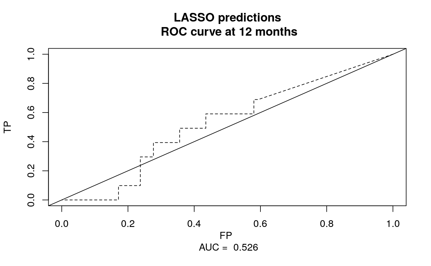
Plot the ROC curve:
library(survivalROC)
nobs <- length(preds)
cutoff <- 12
preds.roc <-
  survivalROC(
    Stime = beer.survival$os,
    status = beer.survival$status,
    marker = preds,
    predict.time = cutoff,
    span = 0.01 * nobs ^ (-0.20)
  )
plot(
  preds.roc$FP,
  preds.roc$TP,
  type = "l",
  xlim = c(0, 1),
  ylim = c(0, 1),
  xlab = paste("FP", "\n", "AUC = ", round(preds.roc$AUC, 3)),
  lty = 2,
  ylab = "TP",
  main = "LASSO predictions\n ROC curve at 12 months"
)
abline(0, 1)

Figure 1: ROC plot of cross-validated continuous risk predictions at 12 months. Note that the predictions are better if you don’t randomly select 250 genes to start with! We only did this to ease the load on the CRAN checking servers.
Getting coefficients for model fit on all the data
Finally, we can get coefficients for the model fit on all the data, for future use. Note that nsim should ideally be greater than 1, to train the model using multiple foldings for cross-validation. The output of opt1D or opt2D will be a matrix with one row per simulation. The default behavior in opt.nested.crossval() is to take the simulation with highest cross-validated partial log likelihood (CVL), which is the recommended way to select a model from the multiple simulations.
beer.coefs <- opt1D(
  setpen = "L1",
  nsim = 1,
  response = surv.obj,
  penalized = dat.filt,
  fold = 5,
  maxlambda1 = 5,
  positive = FALSE,
  standardize = TRUE,
  trace = FALSE
)
We can also include unpenalized covariates, if desired. Note that when keeping only one variable for a penalized or unpenalized covariate, indexing a dataframe like [1] instead of doing [, 1] preserves the variable name. With [, 1] the variable name gets converted to "".
beer.coefs.unpen <-
  opt1D(
    setpen = "L1",
    nsim = 1,
    response = surv.obj,
    penalized = dat.filt[-1],
    # This is equivalent to dat.filt[,-1]
    unpenalized = dat.filt[1],
    fold = 5,
    maxlambda1 = 5,
    positive = FALSE,
    standardize = TRUE,
    trace = FALSE
  )
Note the non-zero first coefficient this time, due to it being unpenalized:
beer.coefs[1, 1:5] #example output with no unpenalized covariates
##             L1            cvl    J04130_s_at U20758_rna1_at    L11672_r_at
## 4.99896033 -115.19258054 0.00000000 0.09998177 -0.10312924beer.coefs.unpen[1, 1:5] #example output with first covariate unpenalized
##             L1            cvl    J04130_s_at U20758_rna1_at    L11672_r_at
##     4.99906823  -117.76317249    -0.15193598     0.10888431    -0.03394335
Simulation of collinear high-dimensional data with survival or binary outcome
The pensim also provides a convenient means to simulation high-dimensional expression data with (potentially censored) survival outcome or binary outcome which is dependent on specified covariates.
Binary outcome example
First, generate the data. Here we simulate 20 variables. The first 15 (group “a”) are uncorrelated, and have no association with outcome. The final five (group “b”) have covariance of 0.8 to each other variable in that group. The response variable is associated with the first variable group “b” (firstonly=TRUE) with a coefficient of 2.
Binary outcomes for \(n_s= 50\) samples are simulated as a Bernoulli distribution with probability for patient s:
\[\begin{equation} p_{s} =\frac{1}{1 + exp(-\beta X_{s})} \end{equation}\]
with \(\beta_{s,16} = 0.5\) and all other \(\beta_{s,i}\) equal to zero.
The code for this simulation is as follows:
set.seed(9)
x <- create.data(
  nvars = c(15, 5),
  cors = c(0, 0.8),
  associations = c(0, 2),
  firstonly = c(TRUE, TRUE),
  nsamples = 50,
  response = "binary",
  logisticintercept = 0.5
)
Take a look at the simulated data:
summary(x)
##              Length Class      Mode
## summary        6    data.frame list
## associations  20    -none-     numeric
## covariance   400    -none-     numeric
## data 21 data.frame listx$summary
##   start end cors associations num firstonly
## a     1  15  0.0            0  15      TRUE
## b    16  20  0.8            2   5      TRUE
A simple logistic model fails at variable selection in this case:
simplemodel <- glm(outcome ~ ., data = x$data, family = binomial)
## Warning: glm.fit: algorithm did not converge## Warning: glm.fit: fitted probabilities numerically 0 or 1 occurredsummary(simplemodel)
##
## Call:
## glm(formula = outcome ~ ., family = binomial, data = x$data)
##
## Deviance Residuals:
##        Min          1Q      Median          3Q         Max
## -2.156e-04  -2.100e-08   2.100e-08   4.490e-06   2.110e-04
##
## Coefficients:
##               Estimate Std. Error z value Pr(>|z|)
## (Intercept)    394.817  40723.092   0.010    0.992
## a.1             -2.017   8340.192   0.000    1.000
## a.2           1054.116 107650.687   0.010    0.992
## a.3            432.929  41344.208   0.010    0.992
## a.4            187.507  21631.886   0.009    0.993
## a.5           -403.302  39003.798  -0.010    0.992
## a.6           -236.102  20862.924  -0.011    0.991
## a.7           -258.201  23085.549  -0.011    0.991
## a.8              7.364  18988.262   0.000    1.000
## a.9            229.596  21020.703   0.011    0.991
## a.10          -519.764  55465.620  -0.009    0.993
## a.11          -718.759  73461.234  -0.010    0.992
## a.12            94.096  16745.928   0.006    0.996
## a.13          -619.513  65350.574  -0.009    0.992
## a.14           585.887  61785.544   0.009    0.992
## a.15          -271.199  30368.663  -0.009    0.993
## b.1            447.844  49587.944   0.009    0.993
## b.2           -100.723  21001.800  -0.005    0.996
## b.3           -197.254  35209.129  -0.006    0.996
## b.4           1540.346 146783.886   0.010    0.992
## b.5          -1080.818 105901.366  -0.010    0.992
##
## (Dispersion parameter for binomial family taken to be 1)
##
##     Null deviance: 6.6406e+01  on 49  degrees of freedom
## Residual deviance: 3.7489e-07  on 29  degrees of freedom
## AIC: 42
##
## Number of Fisher Scoring iterations: 25
But LASSO does a better job, selecting several of the collinear variables in the “b” group of variables which are associated with outcome:
lassofit <-
  opt1D(
    nsim = 3,
    nprocessors = 1,
    setpen = "L1",
    penalized = x$data[1:20],
    response = x$data[, "outcome"],
    trace = FALSE,
    fold = 10
  )
print(lassofit)
##            L1       cvl (Intercept) a.1        a.2 a.3 a.4 a.5         a.6 a.7
## [1,] 4.404100 -32.62007   0.5318400   0 0.04073869   0   0   0 -0.08727491   0
## [2,] 4.992938 -34.51760   0.5204535   0 0.01012467   0   0   0 -0.02152966   0
## [3,] 4.133468 -33.02222   0.5429307   0 0.06228851   0   0   0 -0.11206135   0
##      a.8 a.9        a.10       a.11 a.12 a.13 a.14 a.15        b.1 b.2 b.3
## [1,]   0   0 -0.00379697 -0.3295077    0    0    0    0 0.00000000   0   0
## [2,]   0   0  0.00000000 -0.2793558    0    0    0    0 0.00000000   0   0
## [3,]   0   0 -0.02862559 -0.3483136    0    0    0    0 0.05135596   0   0
##            b.4       b.5
## [1,] 0.2525967 0.1969338
## [2,] 0.2313165 0.1668551
## [3,] 0.2559668 0.1831810
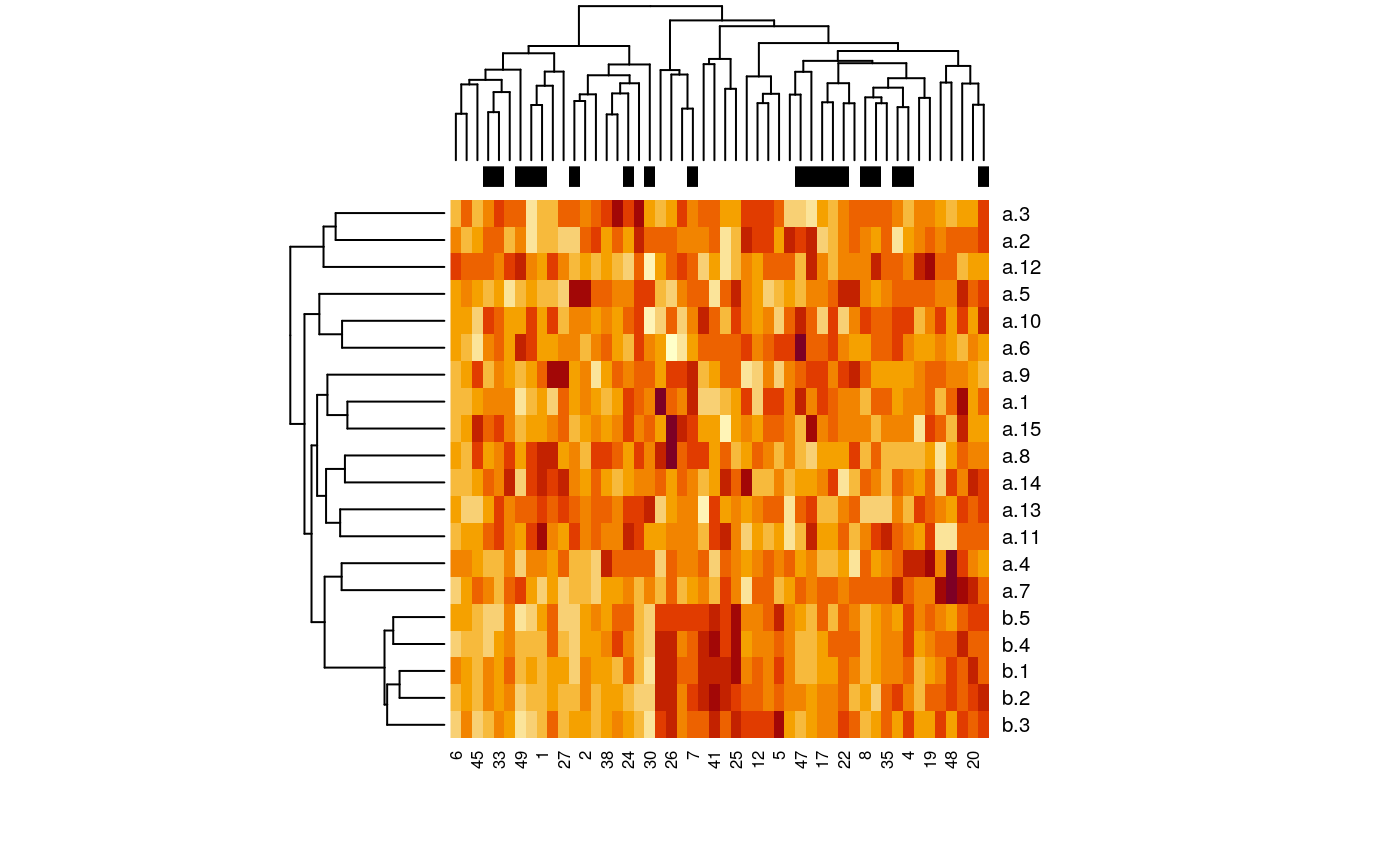
And visualize the data as a heatmap:
dat <- t(as.matrix(x$data[,-match("outcome", colnames(x$data))]))
heatmap(dat, ColSideColors = ifelse(x$data$outcome == 0, "black", "white"))

Figure 2: Heatmap of simulated data with binary response.
Survival outcome example
We simulate these data in the same way, but with response="timetoevent". Here censoring is uniform random between times 2 and 10, generating approximately 34% censoring:
set.seed(1)
x <- create.data(
  nvars = c(15, 5),
  cors = c(0, 0.8),
  associations = c(0, 0.5),
  firstonly = c(TRUE, TRUE),
  nsamples = 50,
  censoring = c(2, 10),
  response = "timetoevent"
)
How many events are censored?
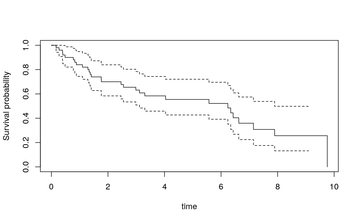
## [1] 0.42Kaplan-Meier plot of this simulated cohort:
library(survival)
surv.obj <- Surv(x$data$time, x$data$cens)
plot(survfit(surv.obj ~ 1), ylab = "Survival probability", xlab = "time")

Figure 3: Kaplan-Meier plot of survival of simulated cohort.
Session Info
## R Under development (unstable) (2020-01-28 r77738)
## Platform: x86_64-pc-linux-gnu (64-bit)
## Running under: Debian GNU/Linux 10 (buster)
##
## Matrix products: default
## BLAS/LAPACK: /usr/lib/x86_64-linux-gnu/libopenblasp-r0.3.5.so
##
## locale:
##  [1] LC_CTYPE=en_US.UTF-8       LC_NUMERIC=C
##  [3] LC_TIME=en_US.UTF-8        LC_COLLATE=en_US.UTF-8
##  [5] LC_MONETARY=en_US.UTF-8    LC_MESSAGES=C
##  [7] LC_PAPER=en_US.UTF-8       LC_NAME=C
##  [9] LC_ADDRESS=C               LC_TELEPHONE=C
## [11] LC_MEASUREMENT=en_US.UTF-8 LC_IDENTIFICATION=C
##
## attached base packages:
## [1] stats     graphics  grDevices utils     datasets  methods   base
##
## other attached packages:
## [1] survivalROC_1.0.3 penalized_0.9-51  survival_3.1-8    pensim_1.2.9
##
## loaded via a namespace (and not attached):
##  [1] Rcpp_1.0.3       knitr_1.28       magrittr_1.5     splines_4.0.0
##  [5] MASS_7.3-51.5    lattice_0.20-40  R6_2.4.1         rlang_0.4.5
##  [9] highr_0.8        stringr_1.4.0    tools_4.0.0      grid_4.0.0
## [13] parallel_4.0.0   xfun_0.12        htmltools_0.4.0  yaml_2.2.1
## [17] assertthat_0.2.1 digest_0.6.25    rprojroot_1.3-2  pkgdown_1.5.0
## [21] crayon_1.3.4     Matrix_1.2-18    fs_1.3.2         memoise_1.1.0
## [25] evaluate_0.14    rmarkdown_2.1    stringi_1.4.6    compiler_4.0.0
## [29] desc_1.2.0       backports_1.1.5
References
Beer, David G., Sharon L.R. Kardia, Chiang-Ching Huang, Thomas J. Giordano, Albert M. Levin, David E. Misek, Lin Lin, et al. 2002. “Gene-Expression Profiles Predict Survival of Patients with Lung Adenocarcinoma.” Nat Med 8 (8): 816–24. https://doi.org/10.1038/nm733.
Goeman, Jelle J. 2010. “L1 Penalized Estimation in the Cox Proportional Hazards Model.” Biometrical Journal. Biometrische Zeitschrift 52 (1): 70–84. https://doi.org/10.1002/bimj.200900028.
Waldron, Levi, Melania Pintilie, Ming-Sound Tsao, Frances A Shepherd, Curtis Huttenhower, and Igor Jurisica. 2011. “Optimized Application of Penalized Regression Methods to Diverse Genomic Data.” Bioinformatics 27 (24): 3399–3406. https://doi.org/10.1093/bioinformatics/btr591.