subtypeHeterogeneity.RmdSetup
library(subtypeHeterogeneity)
library(consensusOV)
library(RaggedExperiment)
library(curatedTCGAData)
library(DropletUtils)
library(ComplexHeatmap)
library(ggplot2)
library(EnrichmentBrowser)
library(curatedTCGAData)
library(DropletUtils)
Data sources
Cancer types
TCGAutils::diseaseCodes[,c("Study.Abbreviation", "Study.Name")]
##    Study.Abbreviation
## 1                 ACC
## 2                BLCA
## 3                BRCA
## 4                CESC
## 5                CHOL
## 6                CNTL
## 7                COAD
## 8                DLBC
## 9                ESCA
## 10               FPPP
## 11                GBM
## 12               HNSC
## 13               KICH
## 14               KIRC
## 15               KIRP
## 16               LAML
## 17               LCML
## 18                LGG
## 19               LIHC
## 20               LUAD
## 21               LUSC
## 22               MESO
## 23               MISC
## 24                 OV
## 25               PAAD
## 26               PCPG
## 27               PRAD
## 28               READ
## 29               SARC
## 30               SKCM
## 31               STAD
## 32               TGCT
## 33               THCA
## 34               THYM
## 35               UCEC
## 36                UCS
## 37                UVM
##                                                          Study.Name
## 1                                          Adrenocortical carcinoma
## 2                                      Bladder Urothelial Carcinoma
## 3                                         Breast invasive carcinoma
## 4  Cervical squamous cell carcinoma and endocervical adenocarcinoma
## 5                                                Cholangiocarcinoma
## 6                                                          Controls
## 7                                              Colon adenocarcinoma
## 8                   Lymphoid Neoplasm Diffuse Large B-cell Lymphoma
## 9                                              Esophageal carcinoma
## 10                                              FFPE Pilot Phase II
## 11                                          Glioblastoma multiforme
## 12                            Head and Neck squamous cell carcinoma
## 13                                               Kidney Chromophobe
## 14                                Kidney renal clear cell carcinoma
## 15                            Kidney renal papillary cell carcinoma
## 16                                           Acute Myeloid Leukemia
## 17                                     Chronic Myelogenous Leukemia
## 18                                         Brain Lower Grade Glioma
## 19                                   Liver hepatocellular carcinoma
## 20                                              Lung adenocarcinoma
## 21                                     Lung squamous cell carcinoma
## 22                                                     Mesothelioma
## 23                                                    Miscellaneous
## 24                                Ovarian serous cystadenocarcinoma
## 25                                        Pancreatic adenocarcinoma
## 26                               Pheochromocytoma and Paraganglioma
## 27                                          Prostate adenocarcinoma
## 28                                            Rectum adenocarcinoma
## 29                                                          Sarcoma
## 30                                          Skin Cutaneous Melanoma
## 31                                           Stomach adenocarcinoma
## 32                                      Testicular Germ Cell Tumors
## 33                                                Thyroid carcinoma
## 34                                                          Thymoma
## 35                             Uterine Corpus Endometrial Carcinoma
## 36                                           Uterine Carcinosarcoma
## 37                                                   Uveal Melanoma
ABSOLUTE
data.dir <- system.file("extdata", package="subtypeHeterogeneity")
absFile <- file.path(data.dir, "ABSOLUTE_grangeslist.rds")
absGRL <- readRDS(absFile)
absGRL
## GRangesList object of length 10803:
## $`TCGA-02-0001-01`
## GRanges object with 59 ranges and 3 metadata columns:
##        seqnames             ranges strand | Modal_HSCN_1 Modal_HSCN_2     score
##           <Rle>          <IRanges>  <Rle> |    <numeric>    <numeric> <integer>
##    [1]     chr1   3218923-74907316      * |            2            2         0
##    [2]     chr1  74918027-75377480      * |            0            2         0
##    [3]     chr1 75377891-247812431      * |            2            2         1
##    [4]     chr2    499482-57091538      * |            2            3         0
##    [5]     chr2  57097020-74690378      * |            0            2         0
##    ...      ...                ...    ... .          ...          ...       ...
##   [55]    chr19  10050184-58866434      * |            1            2         0
##   [56]    chr20    456452-53835558      * |            0            2         1
##   [57]    chr20  53845647-62219837      * |            2            2         1
##   [58]    chr21  15372509-47678774      * |            2            3         0
##   [59]    chr22  17423930-49331012      * |            1            2         0
##   -------
##   seqinfo: 22 sequences from an unspecified genome; no seqlengths
##
## ...
## <10802 more elements>
GISTIC2
gisticOV <- gistic2RSE(ctype="OV", peak="wide")
gisticOV
## class: RangedSummarizedExperiment
## dim: 70 579
## metadata(0):
## assays(1): counts
## rownames: NULL
## rowData names(1): type
## colnames(579): TCGA-04-1331-01 TCGA-04-1332-01 ... TCGA-VG-A8LO-01
##   TCGA-WR-A838-01
## colData names(0):rowRanges(gisticOV)
## GRanges object with 70 ranges and 1 metadata column:
##        seqnames              ranges strand |          type
##           <Rle>           <IRanges>  <Rle> |   <character>
##    [1]     chr1   26963410-27570286      * |      Deletion
##    [2]     chr1   39887948-40168864      * | Amplification
##    [3]     chr1 150483517-150739128      * | Amplification
##    [4]     chr1 207316102-220705691      * |      Deletion
##    [5]     chr1 234417530-235727932      * | Amplification
##    ...      ...                 ...    ... .           ...
##   [66]    chr20   30061713-30332464      * | Amplification
##   [67]    chr20   62137482-63025520      * | Amplification
##   [68]    chr21   42519390-48129895      * |      Deletion
##   [69]    chr22   30113489-30692352      * | Amplification
##   [70]    chr22   48668761-51304566      * |      Deletion
##   -------
## seqinfo: 23 sequences from an unspecified genome; no seqlengthsassay(gisticOV)[1:5,1:5]
##      TCGA-04-1331-01 TCGA-04-1332-01 TCGA-04-1335-01 TCGA-04-1336-01
## [1,]               1               0               1               0
## [2,]               0               1               0               1
## [3,]               1               1               0               0
## [4,]               0               0               0               0
## [5,]               2               0               0               0
##      TCGA-04-1337-01
## [1,]               1
## [2,]               0
## [3,]               0
## [4,]               0
## [5,]               0
Expression-based subtypes
Broad subtypes
ovsubs <- getBroadSubtypes(ctype="OV", clust.alg="CNMF")
dim(ovsubs)
## [1] 569 2head(ovsubs)
##                 cluster silhouetteValue
## TCGA-04-1331-01       1      0.07993633
## TCGA-04-1341-01       1      0.04587895
## TCGA-04-1342-01       1      0.09203928
## TCGA-04-1347-01       1      0.02585325
## TCGA-04-1350-01       1      0.26985422
## TCGA-04-1351-01 1 0.26021068table(ovsubs[,"cluster"])
##
##   1   2   3   4
## 183 114 120 152
OV subtypes from different studies
pooled.file <- file.path(data.dir, "pooled_subtypes.rds")
pooled.subs <- readRDS(pooled.file)
table(pooled.subs[,"data.source"])
##
##   E.MTAB.386     GSE13876     GSE14764     GSE17260     GSE18520     GSE26193
##          128           95           41           43           48           45
##     GSE26712     GSE32062     GSE49997     GSE51088      GSE9891 PMID17290060
##          174          128          122           78          139           56
##         TCGA
## 448table(pooled.subs[,"Verhaak"])
##
## IMR DIF PRO MES
## 441 450 309 345
TCGA subtype consistency
tab <- mapOVSubtypes(ovsubs, pooled.subs)
tab
##      1  2  3  4
## IMR 17 21 18 98
## DIF 26  5 66 16
## PRO 85  5  7  3
## MES 11 62 7 1## PRO MES DIF IMR
## 1 2 3 4sts <- names(ind)[ovsubs[,"cluster"]] ovsubs <- data.frame(ovsubs, subtype=sts, stringsAsFactors=FALSE)
Subtype purity & ploidy
pp.file <- file.path(data.dir, "ABSOLUTE_Purity_Ploidy.rds")
puri.ploi <- readRDS(pp.file)
head(puri.ploi)
##                 purity ploidy Genome.doublings Subclonal.genome.fraction
## TCGA-04-1331-01   0.88   1.85                0                      0.19
## TCGA-04-1341-01   0.82   2.79                1                      0.32
## TCGA-04-1342-01   0.79   2.35                0                      0.23
## TCGA-04-1347-01   0.94   4.29                2                      0.46
## TCGA-04-1350-01   0.99   3.04                1                        NA
## TCGA-04-1351-01 0.72 4.37 2 NAplotSubtypePurityPloidy(ovsubs, puri.ploi)

Assessing the significance of differences between subtypes:
cids <- intersect(rownames(ovsubs), rownames(puri.ploi))
subtys <- ovsubs[cids, "cluster"]
subtys <- names(stcols)[subtys]
pp <- puri.ploi[cids, ]
summary(aov(purity ~ subtype,
            data.frame(purity=pp[,"purity"], subtype=subtys)))
##              Df Sum Sq Mean Sq F value Pr(>F)
## subtype       3  4.244   1.415   109.1 <2e-16 ***
## Residuals   511  6.626   0.013
## ---
## Signif. codes:  0 '***' 0.001 '**' 0.01 '*' 0.05 '.' 0.1 ' ' 1
## 7 observations deleted due to missingnesssummary(aov(ploidy ~ subtype, data.frame(ploidy=pp[,"ploidy"], subtype=subtys)))
##              Df Sum Sq Mean Sq F value Pr(>F)
## subtype       3   14.4   4.792   4.807 0.0026 **
## Residuals   511  509.4   0.997
## ---
## Signif. codes:  0 '***' 0.001 '**' 0.01 '*' 0.05 '.' 0.1 ' ' 1
## 7 observations deleted due to missingnesssummary(aov(subcl ~ subtype, data.frame(subcl=pp[,"Subclonal.genome.fraction"], subtype=subtys)))
##              Df Sum Sq Mean Sq F value Pr(>F)
## subtype       3  0.322 0.10728   4.496 0.0041 **
## Residuals   365  8.708 0.02386
## ---
## Signif. codes:  0 '***' 0.001 '**' 0.01 '*' 0.05 '.' 0.1 ' ' 1
## 153 observations deleted due to missingnesschisq.test(pp[,"Genome.doublings"], subtys)
##
##  Pearson's Chi-squared test
##
## data:  pp[, "Genome.doublings"] and subtys
## X-squared = 28.319, df = 6, p-value = 8.182e-05
Stratifying by purity:
sebin <- stratifyByPurity(ovsubs, puri.ploi, method="equal.bin")
lengths(sebin)
## (0.209,0.368] (0.368,0.526] (0.526,0.684] (0.684,0.842]     (0.842,1]
##             4            36            79           199           197
squint <- stratifyByPurity(ovsubs, puri.ploi, method="quintile") lengths(squint)
## (0.21,0.658] (0.658,0.77]  (0.77,0.84]   (0.84,0.9]      (0.9,1]
##          102          112          103           95          102
Subtype association
pvals <- testSubtypes(gisticOV, ovsubs, padj.method="none")
adj.pvals <- p.adjust(pvals, method="BH")
length(adj.pvals)
## [1] 70head(adj.pvals)
## [1] 0.80025111 0.14279265 0.11317350 0.90288094 0.03365597 0.45058975sum(adj.pvals < 0.1)
## [1] 35hist(pvals, breaks=25, col="firebrick", xlab="Subtype association p-value", main="")

Genomic distribution of subtype-associated CNAs
cnv.genes <- getCnvGenesFromTCGA()
sig.ind <- adj.pvals < 0.1
mcols(gisticOV)$subtype <- testSubtypes(gisticOV, ovsubs, what="subtype")
mcols(gisticOV)$significance <- ifelse(sig.ind, "*", "")
circosSubtypeAssociation(gisticOV, cnv.genes)

plotNrCNAsPerSubtype(mcols(gisticOV)$type[sig.ind], mcols(gisticOV)$subtype[sig.ind])

Annotate cytogenetic bands:
bands.file <- file.path(data.dir, "cytoBand_hg19.txt")
cbands <- read.delim(bands.file, header=FALSE)
cbands <- cbands[,-5]
colnames(cbands) <- c("seqnames", "start", "end", "band")
cbands[,4] <- paste0(sub("^chr", "", cbands[,1]), cbands[,4])
cbands <- makeGRangesFromDataFrame(cbands, keep.extra.columns=TRUE)
genome(cbands) <- "hg19"
cbands
## GRanges object with 862 ranges and 1 metadata column:
##         seqnames            ranges strand |        band
##            <Rle>         <IRanges>  <Rle> | <character>
##     [1]     chr1         0-2300000      * |     1p36.33
##     [2]     chr1   2300000-5400000      * |     1p36.32
##     [3]     chr1   5400000-7200000      * |     1p36.31
##     [4]     chr1   7200000-9200000      * |     1p36.23
##     [5]     chr1  9200000-12700000      * |     1p36.22
##     ...      ...               ...    ... .         ...
##   [858]     chrY 15100000-19800000      * |    Yq11.221
##   [859]     chrY 19800000-22100000      * |    Yq11.222
##   [860]     chrY 22100000-26200000      * |    Yq11.223
##   [861]     chrY 26200000-28800000      * |     Yq11.23
##   [862]     chrY 28800000-59373566      * |        Yq12
##   -------
##   seqinfo: 24 sequences from hg19 genome; no seqlengths
gisticOV <- annotateCytoBands(gisticOV, cbands) mcols(gisticOV)
## DataFrame with 70 rows and 4 columns
##              type   subtype significance        band
##       <character> <integer>  <character> <character>
## 1        Deletion         2                  1p36.11
## 2   Amplification         1                   1p34.3
## 3   Amplification         2                   1q21.3
## 4        Deletion         1                     1q41
## 5   Amplification         1            *      1q42.3
## ...           ...       ...          ...         ...
## 66  Amplification         1            *    20q11.21
## 67  Amplification         1            *    20q13.33
## 68       Deletion         1                  21q22.3
## 69  Amplification         4                  22q12.2
## 70       Deletion         1            *    22q13.33
coocc <- analyzeCooccurence(gisticOV) rownames(coocc) <- mcols(gisticOV)$band ComplexHeatmap::Heatmap(coocc, show_row_names=TRUE, show_column_names=FALSE, column_title="SCNAs", row_title="SCNAs", name="Co-occurrence", row_names_gp = gpar(fontsize = 8))

Subclonality
Match subtyped samples and ABSOLUTE samples
raOV <- getMatchedAbsoluteCalls(absGRL, ovsubs)
raOV
## class: RaggedExperiment
## dim: 76062 516
## assays(3): Modal_HSCN_1 Modal_HSCN_2 score
## rownames: NULL
## colnames(516): TCGA-04-1331-01 TCGA-04-1341-01 ... TCGA-61-2094-01
##   TCGA-61-2104-01
## colData names(3): cluster silhouetteValue subtyperowRanges(raOV)
## GRanges object with 76062 ranges and 0 metadata columns:
##           seqnames              ranges strand
##              <Rle>           <IRanges>  <Rle>
##       [1]     chr1    3218923-32621239      *
##       [2]     chr1   32661059-45934562      *
##       [3]     chr1   45935056-55443605      *
##       [4]     chr1 117773202-117884055      *
##       [5]     chr1 172450760-172879023      *
##       ...      ...                 ...    ...
##   [76058]    chr21   43587562-47678774      *
##   [76059]    chr22   17423930-28566725      *
##   [76060]    chr22   28586674-38703589      *
##   [76061]    chr22   38708404-47224129      *
##   [76062]    chr22   47227321-49331012      *
##   -------
##   seqinfo: 22 sequences from an unspecified genome; no seqlengths
Summarize subclonality of ABSOLUTE calls in GISTIC regions
subcl.gisticOV <- querySubclonality(raOV, query=rowRanges(gisticOV), sum.method="any", ext=500000)
dim(subcl.gisticOV)
## [1] 70 516subcl.gisticOV[1:5,1:5]
##                          TCGA-04-1331-01 TCGA-04-1341-01 TCGA-04-1342-01
## chr1:26463410-28070286                 0               0              NA
## chr1:39387948-40668864                 0               0               0
## chr1:149983517-151239128              NA               1               1
## chr1:206816102-221205691               1               1               1
## chr1:233917530-236227932               1               1               1
##                          TCGA-04-1347-01 TCGA-04-1350-01
## chr1:26463410-28070286                 1               0
## chr1:39387948-40668864                 1               0
## chr1:149983517-151239128               1               0
## chr1:206816102-221205691               1               0
## chr1:233917530-236227932               1               0
Subclonality score
Def: Fraction of samples in which a mutation is subclonal.
## Min. 1st Qu. Median Mean 3rd Qu. Max.
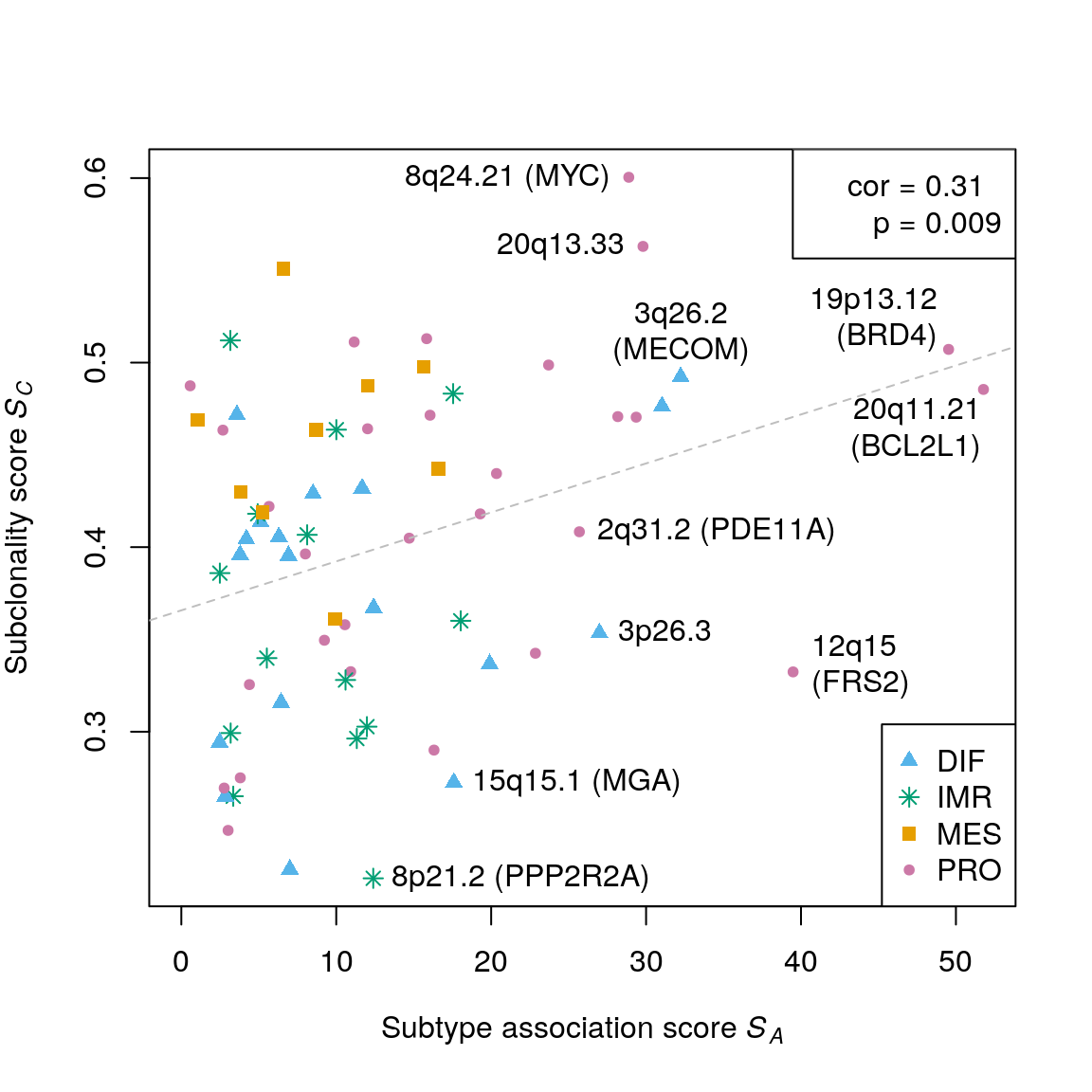
## 0.2206 0.3336 0.4075 0.4009 0.4707 0.6004Correlation: subtype-association score and subclonality score
assoc.score <- testSubtypes(gisticOV, ovsubs, what="statistic")
cor(assoc.score, subcl.score, method="spearman")
## [1] 0.3097017cor.test(assoc.score, subcl.score, method="spearman", exact=FALSE)$p.value
## [1] 0.009081272Permutation test:
obs.cor <- cor(assoc.score, subcl.score, method="spearman")
perm.cor <- replicate(1000,
    cor(sample(assoc.score), subcl.score, method="spearman"))
(sum(perm.cor >= obs.cor) + 1) / (1000 + 1)
## [1] 0.003996004plotCorrelation(assoc.score, subcl.score, subtypes=mcols(gisticOV)$subtype, stcols=stcols[c(4,3,1,2)]) text(x=52.8, y=0.46, "20q11.21\n(BCL2L1)", pos=2) text(x=50, y=0.52, "19p13.12\n(BRD4)", pos=2) text(x=39.489, y=0.332, "12q15\n(FRS2)", pos=4) text(x=32.232, y=0.492, "3q26.2\n(MECOM)", pos=3) text(x=28.883, y=0.6, "8q24.21 (MYC)", pos=2) text(x=29.801, y=0.563, "20q13.33", pos=2) text(x=25.693, y=0.408, "2q31.2 (PDE11A)", pos=4) text(x=26.991, y=0.353, "3p26.3", pos=4) text(x=17.59, y=0.272, "15q15.1 (MGA)", pos=4) text(x=12.389, y=0.22, "8p21.2 (PPP2R2A)", pos=4)
Purity-stratified analysis
sapply(squint, function(ids) analyzeStrata(ids, absGRL, gisticOV, ovsubs))
## (0.21,0.658] (0.658,0.77]  (0.77,0.84]   (0.84,0.9]      (0.9,1]
## 0.2804451 0.3909148 0.1793591 0.2038877 0.2316690sapply(sebin[-1], function(ids) analyzeStrata(ids, absGRL, gisticOV, ovsubs))
## (0.368,0.526] (0.526,0.684] (0.684,0.842]     (0.842,1]
## 0.2298369 0.1667571 0.2469272 0.3788186plotPurityStrata(puri.ploi, ovsubs, gisticOV, absGRL)

plotPurityStrata(puri.ploi, ovsubs, gisticOV, absGRL, method="quintile")

rowRanges(gisticOV)$adj.pval <- adj.pvals
rowRanges(gisticOV)$subcl <- subcl.score
Assessing subclonality calls with PureCN
Read and order
ppp.file <- file.path(data.dir, "PureCN_Purity_Ploidy.txt")
puriploi.pcn <- read.table(ppp.file)
puriploi.pcn <- puriploi.pcn[!duplicated(puriploi.pcn[,1]),]
rownames(puriploi.pcn) <- puriploi.pcn[,"Sampleid"]
puriploi.pcn <- puriploi.pcn[,-1]
puriploi.pcn <- as.matrix(puriploi.pcn)
absdiff <- abs(puriploi.pcn[,c("purity", "ploidy")] -
                puriploi.pcn[,c("Purity_wes", "Ploidy_wes")])
ind <- do.call(order, as.data.frame(absdiff))
puriploi.pcn <- puriploi.pcn[ind,]
head(puriploi.pcn)
##                 purity ploidy Genome.doublings Subclonal.genome.fraction
## TCGA-29-2427-01   0.69   1.80                0                      0.02
## TCGA-24-2035-01   0.61   1.98                0                      0.05
## TCGA-24-1467-01   0.77   3.98                1                      0.09
## TCGA-61-2012-01   0.58   2.90                1                      0.12
## TCGA-13-0751-01   0.93   2.84                1                      0.10
## TCGA-23-2078-01   0.60   1.98                0                      0.17
##                 Purity_wes Ploidy_wes Purity_snp6 Ploidy_snp6
## TCGA-29-2427-01       0.69   1.804566        0.64    1.805899
## TCGA-24-2035-01       0.61   1.945255          NA          NA
## TCGA-24-1467-01       0.78   4.005017        0.71    4.015652
## TCGA-61-2012-01       0.59   2.868254        0.59    2.864081
## TCGA-13-0751-01       0.92   2.808227          NA          NA
## TCGA-23-2078-01 0.59 1.944129 0.59 1.995981cor(puriploi.pcn[,"purity"], puriploi.pcn[,"Purity_wes"], use="complete.obs")
## [1] 0.7684567cor(puriploi.pcn[,"Purity_wes"], puriploi.pcn[,"Purity_snp6"], use="complete.obs")
## [1] 0.8265775CN concordance with ABSOLUTE
PureCN calls for S0293689 capture kit:
pcn.call.file <- file.path(data.dir, "PureCN_OV_S0293689_grangeslist.rds")
pcn.calls <- readRDS(pcn.call.file)
pcn.calls
## GRangesList object of length 171:
## $`TCGA-13-0924-01`
## GRanges object with 545 ranges and 2 metadata columns:
##     seqnames              ranges strand |        CN     score
##        <Rle>           <IRanges>  <Rle> | <numeric> <integer>
##         chr1       36357-6634553      * |         2         0
##         chr1    6634723-10629753      * |         1         0
##         chr1   10629823-10659920      * |         2         0
##         chr1   10659931-11519947      * |         1         0
##         chr1   11520570-11649964      * |         2         0
##   .      ...                 ...    ... .       ...       ...
##        chr23 153743355-153785541      * |         3         0
##        chr23 153785930-154558727      * |         2         0
##        chr23 154560355-154642787      * |         3         0
##        chr23 154645729-156010146      * |         2         0
##        chr23 156010202-156010468      * |         1         0
##   -------
##   seqinfo: 23 sequences from an unspecified genome; no seqlengths
##
## ...
## <170 more elements>
# select samples that intersect with ABSOLUTE data isect.samples <- intersect(names(pcn.calls), names(absGRL)) pcn.calls <- pcn.calls[isect.samples] pcn.calls.ra <- RaggedExperiment(pcn.calls) pcn.calls.ra
## class: RaggedExperiment
## dim: 185221 166
## assays(2): CN score
## rownames(185221): '' '' ... '' ''
## colnames(166): TCGA-13-0924-01 TCGA-29-1768-01 ... TCGA-29-1784-01
##   TCGA-13-0807-01
## colData names(0):
Get corresponding ABSOLUTE calls:
abs.calls <- absGRL[isect.samples]
abs.calls <- as.data.frame(abs.calls)[,c(2:5,8:10)]
totalCN <- abs.calls[,"Modal_HSCN_1"] + abs.calls[,"Modal_HSCN_2"]
abs.calls <- data.frame(abs.calls[,1:4], CN=totalCN, score=abs.calls[,"score"])
abs.calls <- makeGRangesListFromDataFrame(abs.calls,
    split.field="group_name", keep.extra.columns=TRUE)
abs.calls
## GRangesList object of length 166:
## $`TCGA-04-1332-01`
## GRanges object with 104 ranges and 2 metadata columns:
##         seqnames              ranges strand |        CN     score
##            <Rle>           <IRanges>  <Rle> | <numeric> <integer>
##     [1]     chr1    3218923-34828319      * |         3         0
##     [2]     chr1   34829840-49468025      * |         4         0
##     [3]     chr1 116676668-166002656      * |         4         1
##     [4]     chr1 166002866-196696737      * |         4         1
##     [5]     chr1 196966853-247812431      * |         3         0
##     ...      ...                 ...    ... .       ...       ...
##   [100]    chr20     456452-42230695      * |         3         0
##   [101]    chr20   42240730-62219837      * |         4         0
##   [102]    chr21   15372509-36666340      * |         4         0
##   [103]    chr21   36669447-47678774      * |         4         1
##   [104]    chr22   17423930-32027449      * |         3         0
##   -------
##   seqinfo: 22 sequences from an unspecified genome; no seqlengths
##
## ...
## <165 more elements>
abs.calls.ra <- RaggedExperiment(abs.calls) abs.calls.ra <- abs.calls.ra[,colnames(pcn.calls.ra)]
OVC GISTIC2 regions on hg19 (ABSOLUTE) and hg38 (PureCN)
gisticOV.ranges.hg19 <- file.path(data.dir, "gisticOV_ranges_hg19.txt")
gisticOV.ranges.hg19 <- scan(gisticOV.ranges.hg19, what="character")
gisticOV.ranges.hg19 <- GRanges(gisticOV.ranges.hg19)
gisticOV.ranges.hg19
## GRanges object with 65 ranges and 0 metadata columns:
##        seqnames              ranges strand
##           <Rle>           <IRanges>  <Rle>
##    [1]     chr1   26963410-27570286      *
##    [2]     chr1   39887948-40168864      *
##    [3]     chr1 150483517-150739128      *
##    [4]     chr1 207316102-220705691      *
##    [5]     chr1 234417530-235727932      *
##    ...      ...                 ...    ...
##   [61]    chr20           1-4108014      *
##   [62]    chr20   30061713-30332464      *
##   [63]    chr21   42519390-48129895      *
##   [64]    chr22   30113489-30692352      *
##   [65]    chr22   48668761-51304566      *
##   -------
##   seqinfo: 22 sequences from an unspecified genome; no seqlengths
gisticOV.ranges.hg38 <- file.path(data.dir, "gisticOV_ranges_hg38.txt") gisticOV.ranges.hg38 <- scan(gisticOV.ranges.hg38, what="character") gisticOV.ranges.hg38 <- GRanges(gisticOV.ranges.hg38) gisticOV.ranges.hg38
## GRanges object with 65 ranges and 0 metadata columns:
## seqnames ranges strand
## <Rle> <IRanges> <Rle>
## [1] chr1 26636919-27243795 *
## [2] chr1 39422276-39703192 *
## [3] chr1 150511041-150766652 *
## [4] chr1 207142757-220532349 *
## [5] chr1 234281784-235564632 *
## ... ... ... ...
## [61] chr20 79360-4127367 *
## [62] chr20 31473910-31744661 *
## [63] chr21 41147463-46699983 *
## [64] chr22 29717500-30296363 *
## [65] chr22 48272949-50806138 *
## -------
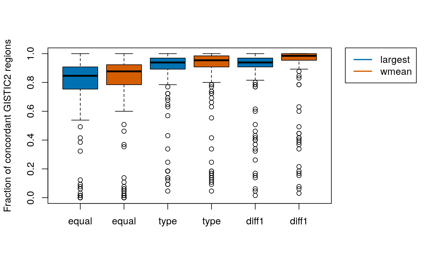
## seqinfo: 22 sequences from an unspecified genome; no seqlengthsSummarize calls in GISTIC regions using either
- the largest call overlapping a GISTIC region
- a weighted mean of calls overlapping a GISTIC region
.largest <- function(score, range, qrange)
{
    return.type <- class(score[[1]])
    default.value <- do.call(return.type, list(1))
    ind <- which.max(width(range))
    res <- vapply(seq_along(score),
           function(i) score[[i]][ind[i]], default.value)
    return(res)
}
pcn.rassay <- qreduceAssay(pcn.calls.ra, query=gisticOV.ranges.hg38,
                    simplifyReduce=.largest, background=2)
abs.rassay <- qreduceAssay(abs.calls.ra, query=gisticOV.ranges.hg19,
                    simplifyReduce=.largest, background=2)


.weightedmean <- function(score, range, qrange)
{
    w <- width(range)
    s <- sum(score * w) / sum(w)
    return(round(s))
}

pcn.rassay2 <- qreduceAssay(pcn.calls.ra, query=gisticOV.ranges.hg38,
                    simplifyReduce=.weightedmean, background=2)
abs.rassay2 <- qreduceAssay(abs.calls.ra, query=gisticOV.ranges.hg19,
                    simplifyReduce=.weightedmean, background=2)
Evaluate per-sample concordance:
- fraction of GISTIC regions with equal copy number
- fraction of GISTIC regions agreeing in alteration type (amplification / deletion)
- fraction of GISTIC regions that deviate by max. 1 copy
# largest
fract.equal <- vapply(seq_along(isect.samples),
        function(i) mean(pcn.rassay[,i] == abs.rassay[,i]),
        numeric(1))
fract.type <- vapply(seq_along(isect.samples),
        function(i) mean(((pcn.rassay[,i] < 2) & (abs.rassay[,i] < 2)) |
                          ((pcn.rassay[,i] > 2) & (abs.rassay[,i] > 2)) |
                          ((pcn.rassay[,i] == 2) & (abs.rassay[,i] == 2))),
        numeric(1))
fract.diff1 <- vapply(seq_along(isect.samples),
        function(i) mean((pcn.rassay[,i] == abs.rassay[,i]) |
                            (pcn.rassay[,i] == abs.rassay[,i] + 1) |
                            (pcn.rassay[,i] == abs.rassay[,i] - 1)),
        numeric(1))

# weighted mean
fract.equal2 <- vapply(seq_along(isect.samples),
        function(i) mean(pcn.rassay2[,i] == abs.rassay2[,i]),
        numeric(1))
fract.type2 <- vapply(seq_along(isect.samples),
        function(i) mean(((pcn.rassay2[,i] < 2) & (abs.rassay2[,i] < 2)) |
                          ((pcn.rassay2[,i] > 2) & (abs.rassay2[,i] > 2)) |
                          ((pcn.rassay2[,i] == 2) & (abs.rassay2[,i] == 2))),
        numeric(1))
fract.diff12 <- vapply(seq_along(isect.samples),
        function(i) mean((pcn.rassay2[,i] == abs.rassay2[,i]) |
                            (pcn.rassay2[,i] == abs.rassay2[,i] + 1) |
                            (pcn.rassay2[,i] == abs.rassay2[,i] - 1)),
        numeric(1))
Plot concordance:
par(mar=c(5.1, 4.1, 4.1, 8.1), xpd=TRUE)
boxplot(fract.equal, fract.equal2,
        fract.type, fract.type2,
        fract.diff1, fract.diff12, col=rep(c(cb.blue, cb.red), 3),
        names=rep(c("equal", "type", "diff1"), each=2),
        ylab="Fraction of concordant GISTIC2 regions")
legend("topright", inset=c(-0.3,0), legend=c("largest", "wmean"),
        col=c(cb.blue, cb.red), lwd=2)
Select large losses called subclonal by ABSOLUTE
selectAbsCalls <- function(sample, min.size=3000000)
{
    gr <- absGRL[[sample]]
    gr.3MB <- width(gr) > min.size
    is.loss <- (gr$Modal_HSCN_1 + gr$Modal_HSCN_2) < 2
    is.subcl <- gr$score == 1

    ind <- gr.3MB & is.loss & is.subcl
    return(gr[ind])
}
(abs.calls <- selectAbsCalls(rownames(puriploi.pcn)[1]))
## GRanges object with 4 ranges and 3 metadata columns:
##       seqnames             ranges strand | Modal_HSCN_1 Modal_HSCN_2     score
##          <Rle>          <IRanges>  <Rle> |    <numeric>    <numeric> <integer>
##   [1]    chr13  49131496-77266538      * |            0            1         1
##   [2]    chr13 78155543-114987333      * |            0            1         1
##   [3]    chr14  23708769-32553018      * |            0            1         1
##   [4]    chr19  15079104-28465910      * |            0            1         1
##   -------
##   seqinfo: 22 sequences from an unspecified genome; no seqlengths
liftOver hg19-based ABSOLUTE calls to compare with hg38-based PureCN calls
- UCSC online liftOver (https://genome.ucsc.edu/cgi-bin/hgLiftOver)
- does smoothing and filtering on top of the chain mappings
-
rtracklayer::liftOveronly provides chain mappings
chain.file <- file.path(data.dir, "hg19ToHg38.over.chain")
ch <- rtracklayer::import.chain(chain.file)
(hg19.call <- absGRL[[1]][1])
## GRanges object with 1 range and 3 metadata columns:
##       seqnames           ranges strand | Modal_HSCN_1 Modal_HSCN_2     score
##          <Rle>        <IRanges>  <Rle> |    <numeric>    <numeric> <integer>
##   [1]     chr1 3218923-74907316      * |            2            2         0
##   -------
## seqinfo: 22 sequences from an unspecified genome; no seqlengths(blocks <- rtracklayer::liftOver(hg19.call, ch))
## GRangesList object of length 1:
## [[1]]
## GRanges object with 1072 ranges and 3 metadata columns:
##          seqnames            ranges strand | Modal_HSCN_1 Modal_HSCN_2
##             <Rle>         <IRanges>  <Rle> |    <numeric>    <numeric>
##      [1]     chr1   3302359-3928704      * |            2            2
##      [2]     chr1   3935210-3936533      * |            2            2
##      [3]     chr1   3936534-7366717      * |            2            2
##      [4]     chr1   7366718-7382536      * |            2            2
##      [5]     chr1   7382538-8504448      * |            2            2
##      ...      ...               ...    ... .          ...          ...
##   [1068]     chr1 13203465-13203520      * |            2            2
##   [1069]     chr1 13203521-13203532      * |            2            2
##   [1070]     chr1 13203533-13203548      * |            2            2
##   [1071]    chr20 38461961-38462015      * |            2            2
##   [1072]     chr1 12893309-12893335      * |            2            2
##              score
##          <integer>
##      [1]         0
##      [2]         0
##      [3]         0
##      [4]         0
##      [5]         0
##      ...       ...
##   [1068]         0
##   [1069]         0
##   [1070]         0
##   [1071]         0
##   [1072]         0
##   -------
##   seqinfo: 2 sequences from an unspecified genome; no seqlengths
blocks <- unlist(blocks) # harmonize chromosome by majority vote tab <- table(as.character(seqnames(blocks))) nmax <- names(tab)[which.max(tab)] # collapse blocks blocks <- blocks[seqnames(blocks) == nmax] (hg38.call <- range(reduce(blocks)))
## GRanges object with 1 range and 0 metadata columns:
##       seqnames           ranges strand
##          <Rle>        <IRanges>  <Rle>
##   [1]     chr1 3302359-74441632      *
##   -------
##   seqinfo: 2 sequences from an unspecified genome; no seqlengths
Select GISTIC regions of high subtype association and subclonality
tests <- testSubtypes(gisticOV, ovsubs, what="full")
extraL <- stratifySubclonality(gisticOV, subcl.gisticOV, ovsubs,
                               tests, st.names = names(stcols)[c(4,3,1,2)])
# highest subtype association
ind <- order(assoc.score, decreasing=TRUE)
rowRanges(gisticOV)[ind[1:2]]
## GRanges object with 2 ranges and 6 metadata columns:
##       seqnames            ranges strand |          type   subtype significance
##          <Rle>         <IRanges>  <Rle> |   <character> <integer>  <character>
##   [1]    chr20 30061713-30332464      * | Amplification         1            *
##   [2]    chr19 15333311-15422141      * | Amplification         1            *
##              band    adj.pval     subcl
##       <character>   <numeric> <numeric>
##   [1]    20q11.21 1.44652e-07  0.485465
##   [2]    19p13.12 2.04648e-07  0.507163
##   -------
##   seqinfo: 23 sequences from an unspecified genome; no seqlengths
# 20q11.21 (BCL2L1) x <- tests[[ind[1]]] (ot <- x$observed)
##    subtys
## x    1  2  3  4
##   0 44 41 72 68
##   1 77 55 32 59
## 2 55 14 14 24x$expected
##    subtys
## x          1        2        3        4
##   0 71.35135 44.59459 47.83784 61.21622
##   1 70.71712 44.19820 47.41261 60.67207
##   2 33.93153 21.20721 22.74955 29.11171
diff <- x$observed - x$expected (csums <- colSums(diff^2 / x$expected))
##         1         2         3         4
## 24.124538  5.378997 20.579286  1.695401
# 19p13.12 (BRD4) x <- tests[[ind[2]]] (ot <- x$observed)
##    subtys
## x    1  2  3  4
##   0 62 67 48 76
##   1 49 36 45 54
## 2 65 7 25 21x$expected
##    subtys
## x          1        2        3        4
##   0 80.23063 50.14414 53.79099 68.83423
##   1 58.34955 36.46847 39.12072 50.06126
##   2 37.41982 23.38739 25.08829 32.10450
diff <- x$observed - x$expected (csums <- colSums(diff^2 / x$expected))
##         1         2         3         4
## 25.968516 17.154615  1.507324  4.896757
# highest subclonality ind <- order(subcl.score, decreasing=TRUE) rowRanges(gisticOV)[ind[1:2]]
## GRanges object with 2 ranges and 6 metadata columns:
##       seqnames              ranges strand |          type   subtype
##          <Rle>           <IRanges>  <Rle> |   <character> <integer>
##   [1]     chr8 128694547-129309687      * | Amplification         1
##   [2]    chr20   62137482-63025520      * | Amplification         1
##       significance        band    adj.pval     subcl
##        <character> <character>   <numeric> <numeric>
##   [1]            *     8q24.21 0.000497912  0.600432
##   [2]            *    20q13.33 0.000428776  0.562982
##   -------
##   seqinfo: 23 sequences from an unspecified genome; no seqlengths
x <- extraL[order(subcl.score, decreasing=TRUE)[c(1,2,7)]] names(x) <- c("8q24.21 (MYC)", c("20q13.33"), c("19p13.12 (BRD4)")) x <- c(x, extraL[order(subcl.score)[c(1,7,9)]]) names(x)[4:6] <- c("8p21.2 (PPP2R2A)", "15q15.1 (MGA)", "15q11.2 (SNRPN)") ggplotSubtypeStrata(x[c(4:6,1:3)], rep(c("loss","gain"), each=3))

Strongest subtype association:
ind <- order(assoc.score, decreasing=TRUE)
x <- extraL[ind[c(1,3:5,7,9)]]
names(x) <- c("20q11.21 (BCL2L1)", "12q15 (FRS2)", "3q26.2 (MECOM)",
    "6p22.3 (ID4)", "20p13", "12p13.33")
ggplotSubtypeStrata(x, rep("gain", 6))

Regions of frequent loss in HGSOC:
x <- extraL[c(34,44,55)]
names(x) <- c("10q23.31 (PTEN)", "13q14.2 (RB1)", "17q11.2 (NF1)")
ggplotSubtypeStrata(x, rep("loss", 3))

Enrichment of deletions in predom. clonal regions
rowRanges(gisticOV)$type[subcl.score < 0.3]
##  [1] "Amplification" "Deletion"      "Deletion"      "Deletion"
##  [5] "Deletion"      "Deletion"      "Deletion"      "Deletion"
##  [9] "Deletion"      "Deletion"      "Deletion"      "Deletion"
Other cancer types
Number of samples
st <- sapply(allCT, function(ct) nrow(ct$subtypes))
gs <- sapply(allCT, function(ct) ncol(ct$gistic))
as <- sapply(allCT, function(ct) sum(rownames(ct$subtypes) %in% names(absGRL)))

plotNrSamples(gs, st, as)

Number of subtypes & GISTIC regions
nr.sts <- sapply(allCT, function(ct) length(unique(ct$subtypes[,1])))
nr.gregs <- sapply(allCT, function(ct) nrow(ct$gistic))
plotNrSubtypesVsNrGisticRegions(nr.sts, nr.gregs)

Subclonality
subcl.scores <- lapply(allCT, function(ct) ct$subcl.score)
plotSubclonalityDistributions(subcl.scores)

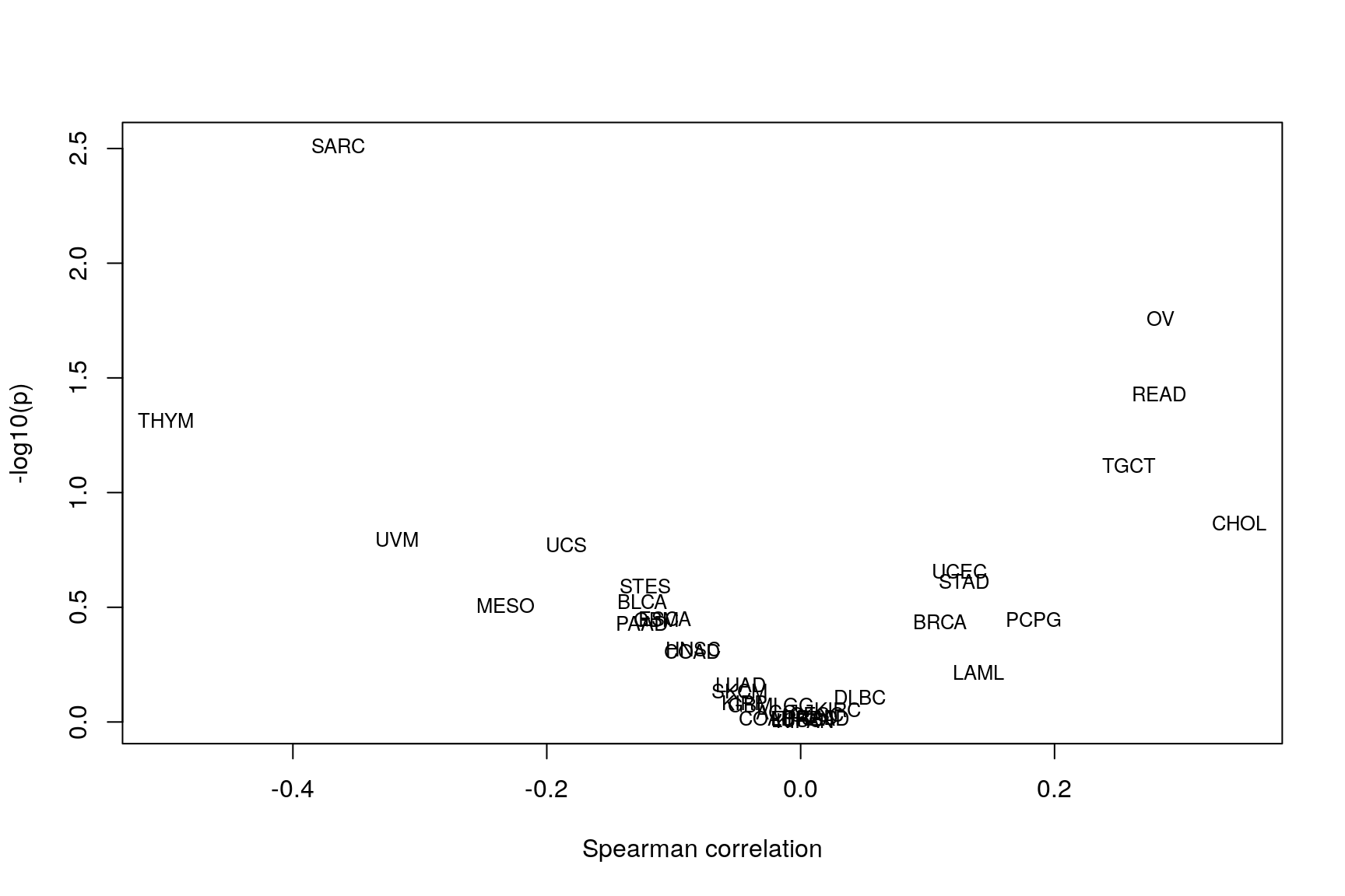
Correlation: subtype association & subclonality
rho <- sapply(allCT, function(ct) ct$rho)
p <- sapply(allCT, function(ct) ct$p)
volcanoCorrelation(rho, p)
Intrinsic subtypes: sarcoma
gisticSARC <- gistic2RSE(ctype="SARC", peak="wide")
sarcsubs <- getBroadSubtypes(ctype="SARC", clust.alg="CNMF")
## Warning in getBroadSubtypes(ctype = "SARC", clust.alg = "CNMF"): mRNA clustering
## not available for SARC - mRNAseq clustering is taken insteadtable(sarcsubs$cluster)
##
##   1   2   3
## 116  78  65
pvals <- suppressWarnings( testSubtypes(gisticSARC, sarcsubs, padj.method="none") ) length(pvals)
## [1] 64## [1] 41hist(pvals, breaks=25, col="firebrick",xlab="Subtype association p-value", main="")

sarc.clin <- RTCGAToolbox::getFirehoseData(dataset="SARC", runDate="20160128")
## gdac.broadinstitute.org_SARC.Clinical_Pick_Tier1.Level_4.2016012800.0.0.tar.gz## gdac.broadinstitute.org_SARC.Clinical_Pick_Tier1.Level_4.2016012800.0.0sarc.clin <- RTCGAToolbox::getData(sarc.clin, "clinical") ids <- rownames(sarcsubs) ids <- tolower(ids) ids <- gsub("-", ".", ids) ids <- substring(ids, 1, 12) sarcsubs$histType <- sarc.clin[ids,"histological_type"] lapply(1:3, function(cl) table(sarcsubs[sarcsubs$cluster == cl,"histType"]))
## [[1]]
##
##                                             dedifferentiated liposarcoma
##                                                                       38
## giant cell 'mfh' / undifferentiated pleomorphic sarcoma with giant cells
##                                                                        1
##                                                     leiomyosarcoma (lms)
##                                                                       12
##                         malignant peripheral nerve sheath tumors (mpnst)
##                                                                        1
##                                                         myxofibrosarcoma
##                                                                       23
##                 pleomorphic 'mfh' / undifferentiated pleomorphic sarcoma
##                                                                       25
##                               undifferentiated pleomorphic sarcoma (ups)
##                                                                       16
##
## [[2]]
##
## dedifferentiated liposarcoma         leiomyosarcoma (lms)
##                            1                           77
##
## [[3]]
##
##                             dedifferentiated liposarcoma
##                                                       19
##                                            desmoid tumor
##                                                        2
##                                     leiomyosarcoma (lms)
##                                                       15
##         malignant peripheral nerve sheath tumors (mpnst)
##                                                        8
##                                         myxofibrosarcoma
##                                                        2
## pleomorphic 'mfh' / undifferentiated pleomorphic sarcoma
##                                                        4
##                 sarcoma; synovial; poorly differentiated
##                                                        2
##                              synovial sarcoma - biphasic
##                                                        2
##                            synovial sarcoma - monophasic
##                                                        6
##               undifferentiated pleomorphic sarcoma (ups)
##                                                        5
assoc.score <- suppressWarnings( testSubtypes(gisticSARC, sarcsubs, what="statistic") ) raSARC <- getMatchedAbsoluteCalls(absGRL, sarcsubs) subcl.gisticSARC <- querySubclonality(raSARC, query=rowRanges(gisticSARC), sum.method="any") subcl.score <- rowMeans(subcl.gisticSARC, na.rm=TRUE) summary(subcl.score)
##    Min. 1st Qu.  Median    Mean 3rd Qu.    Max.
## 0.2486 0.3667 0.4736 0.4701 0.5573 0.6788cor(assoc.score, subcl.score, method="spearman")
## [1] -0.364473cor.test(assoc.score, subcl.score, method="spearman", exact=FALSE)$p.value
## [1] 0.003067494sarc.cols <- stcols[c(1,3,2)] names(sarc.cols) <- c("MFS/UPS", "LMS", "DDLPS") sts <- suppressWarnings( testSubtypes(gisticSARC, sarcsubs, what="subtype") ) sts <- names(sarc.cols)[sts] plotCorrelation(assoc.score, subcl.score, subtypes=sts, stcols=sarc.cols, lpos="right") # top assoc text(x=56.885, y=0.548, "1p36.32\n(TP73)", pos=2) text(x=36.908, y=0.336, "6q25.1\n(UST)", pos=4) text(x=33.943, y=0.275, "10q23.31 (PTEN)", pos=2) text(x=30.257, y=0.249, "13q14.2 (RB1)", pos=2) text(x=27.44, y=0.435, "10q26.3\n(SPRN)", pos=4) text(x=25.501, y=0.362, "1p32.1\n(JUN)", pos=4) # top subcl text(x=10.116, y=0.679, "8q", pos=4) text(x=6.37, y=0.678, "9q34", pos=2) text(x=8.586, y=0.662, "17q", pos=4) text(x=7.658, y=0.65, "5p15.33\n(TERT)", pos=2) text(x=19.497, y=0.625, "8p23.2 (CSMD1)", pos=4) text(x=17.4, y=0.625, "20q13.33", pos=2) text(x=55.915, y=0.262, "12q15 (MDM2)", pos=2)

gisticSARC <- annotateCytoBands(gisticSARC, cbands)
rowRanges(gisticSARC)$assoc.score <- assoc.score
rowRanges(gisticSARC)$subcl <- subcl.score
rowRanges(gisticSARC)$subtype <- sts
ind.assoc <- order(assoc.score, decreasing=TRUE)
ind.subcl <- order(subcl.score, decreasing=TRUE)
rowRanges(gisticSARC)[ind.assoc]
## GRanges object with 64 ranges and 5 metadata columns:
##        seqnames              ranges strand |          type        band
##           <Rle>           <IRanges>  <Rle> |   <character> <character>
##    [1]     chr1           1-5923787      * |      Deletion     1p36.32
##    [2]    chr12   69178021-69244387      * | Amplification       12q15
##    [3]     chr6 148810209-149693136      * | Amplification      6q25.1
##    [4]    chr10   89617158-89755074      * |      Deletion    10q23.31
##    [5]    chr13   48875329-49064807      * |      Deletion     13q14.2
##    ...      ...                 ...    ... .           ...         ...
##   [60]     chr6  66417081-104031403      * |      Deletion      6q14.1
##   [61]    chr11            1-496996      * |      Deletion     11p15.5
##   [62]    chr12 132611527-133851895      * |      Deletion    12q24.33
##   [63]    chr18           1-5145388      * |      Deletion    18p11.32
##   [64]    chr22   45095899-51304566      * |      Deletion    22q13.31
##        assoc.score     subcl     subtype
##          <numeric> <numeric> <character>
##    [1]     56.8853  0.548193         LMS
##    [2]     55.9154  0.261905         LMS
##    [3]     36.9080  0.336000     MFS/UPS
##    [4]     33.9432  0.274510         LMS
##    [5]     30.2573  0.248588       DDLPS
##    ...         ...       ...         ...
##   [60]    1.450279  0.585799       DDLPS
##   [61]    1.238339  0.445205       DDLPS
##   [62]    0.904199  0.500000         LMS
##   [63]    0.742853  0.443709         LMS
##   [64]    0.641115  0.610738       DDLPS
##   -------
## seqinfo: 23 sequences from an unspecified genome; no seqlengthsrowRanges(gisticSARC)[ind.subcl]
## GRanges object with 64 ranges and 5 metadata columns:
##        seqnames              ranges strand |          type        band
##           <Rle>           <IRanges>  <Rle> |   <character> <character>
##    [1]     chr8  54604081-146364022      * | Amplification      8q24.3
##    [2]     chr9 134952380-141213431      * |      Deletion      9q34.3
##    [3]    chr17   57292827-81195210      * | Amplification     17q25.3
##    [4]     chr5           1-5129938      * |      Deletion     5p15.33
##    [5]     chr8           1-4251018      * |      Deletion      8p23.3
##    ...      ...                 ...    ... .           ...         ...
##   [60]     chr3   86917447-87350419      * | Amplification      3p12.1
##   [61]    chr10   89617158-89755074      * |      Deletion    10q23.31
##   [62]     chr8   37911089-38852966      * | Amplification     8p11.22
##   [63]    chr12   69178021-69244387      * | Amplification       12q15
##   [64]    chr13   48875329-49064807      * |      Deletion     13q14.2
##        assoc.score     subcl     subtype
##          <numeric> <numeric> <character>
##    [1]    10.11579  0.678788       DDLPS
##    [2]     6.36997  0.678322         LMS
##    [3]     8.58887  0.664557       DDLPS
##    [4]     7.65827  0.664430         LMS
##    [5]    19.49664  0.625000     MFS/UPS
##    ...         ...       ...         ...
##   [60]    18.08966  0.311475     MFS/UPS
##   [61]    33.94320  0.274510         LMS
##   [62]     3.39771  0.265152     MFS/UPS
##   [63]    55.91538  0.261905         LMS
##   [64]    30.25732  0.248588       DDLPS
##   -------
##   seqinfo: 23 sequences from an unspecified genome; no seqlengths
tests <- suppressWarnings( testSubtypes(gisticSARC, sarcsubs, what="full") ) extraL <- stratifySubclonality(gisticSARC, subcl.gisticSARC, sarcsubs, tests, st.names=names(sarc.cols))
x <- extraL[order(subcl.score)[c(1,2,4)]]
# loss, gain, loss
names(x) <- c("13q14.2 (RB1)", "12q15 (MDM2)", "10q23.31 (PTEN)")
sarc.hscl <- extraL[rowRanges(gisticSARC)$band %in% c("1p36.32", "8p23.3", "20q13.33")]
x <- c(x, sarc.hscl)
# loss, loss, loss
names(x)[4:6] <- c("1p36.32 (TP73)", "8p23.2 (CSMD1)", "20q13.33")
ggplotSubtypeStrata(x, c("loss","gain", rep("loss", 3), "gain"))

Using histopathological classification for subtype assignment:
histcl <- rep(4, nrow(sarcsubs))
ind <- grep("myxofibrosarcoma", sarcsubs$histType)
histcl[ind] <- 1
ind <- grep("undifferentiated pleomorphic sarcoma", sarcsubs$histType)
histcl[ind] <- 1
ind <- grep("leiomyosarcoma", sarcsubs$histType)
histcl[ind] <- 2
ind <- grep("dedifferentiated liposarcoma", sarcsubs$histType)
histcl[ind] <- 3
histsubs <- sarcsubs[histcl != 4,]
histsubs$cluster <- histcl[histcl != 4]
assoc.score <- suppressWarnings( testSubtypes(gisticSARC, histsubs, what="statistic") )
raSARC <- getMatchedAbsoluteCalls(absGRL, histsubs)
subcl.gisticSARC <- querySubclonality(raSARC, query=rowRanges(gisticSARC), sum.method="any")
subcl.score <- rowMeans(subcl.gisticSARC, na.rm=TRUE)
summary(subcl.score)
##    Min. 1st Qu.  Median    Mean 3rd Qu.    Max.
## 0.2308 0.3677 0.4748 0.4713 0.5511 0.6788cor(assoc.score, subcl.score, method="spearman")
## [1] -0.3810298cor.test(assoc.score, subcl.score, method="spearman", exact=FALSE)$p.value
## [1] 0.001894787
Subtype classification in single-cell RNA-seq data
Subtype classification
Genes considered by the consensusOV classifier:
library(consensusOV)
clgenes <- getClassifierGenes()
clgenes
##   [1] "10158"  "10278"  "10395"  "10437"  "10630"  "10635"  "10982"  "11343"
##   [9] "1191"   "1288"   "1289"   "1295"   "1318"   "1490"   "1890"   "1901"
##  [17] "2123"   "2149"   "2207"   "22836"  "22919"  "23022"  "23220"  "2335"
##  [25] "2524"   "259173" "26271"  "27286"  "27299"  "301"    "3268"   "3627"
##  [33] "3902"   "3903"   "3912"   "3925"   "3934"   "3956"   "4038"   "4082"
##  [41] "4162"   "4237"   "4250"   "4261"   "4323"   "4430"   "4681"   "4837"
##  [49] "4921"   "50615"  "51091"  "51177"  "5118"   "54020"  "54587"  "547"
##  [57] "54961"  "55240"  "55340"  "5569"   "55859"  "55930"  "56937"  "57007"
##  [65] "5732"   "5920"   "60489"  "6297"   "64092"  "642"    "6503"   "65108"
##  [73] "65244"  "6602"   "6624"   "6782"   "7216"   "7345"   "7456"   "775"
##  [81] "7805"   "79070"  "79083"  "800"    "81831"  "834"    "83439"  "8460"
##  [89] "84707"  "8522"   "8533"   "8564"   "861"    "8655"   "8764"   "9246"
##  [97] "9447"   "9610"   "9766"   "9854"   "9891"   "9940"   "9961"
Single cell data restricted to classifier genes:
sc.file <- file.path(data.dir, "scRNAseq_consensusOV_genes.txt")
sc.expr <- as.matrix(read.delim(sc.file, row.names=1L))
dim(sc.expr)
## [1] 103 67sc.expr[1:5,1:5]
##       Bulk_2 X1_C01 X1_C02 X1_C03 X1_C08
## 26271  19.62      0      0      0   0.00
## 6782   47.73      0      0      0  79.25
## 57007  93.28      0      0      0   0.00
## 81831   0.00      0      0      0  16.29
## 5569    5.15      0      0      0   0.00
# exclude all zero ind <- apply(sc.expr, 1, function(x) all(x == 0)) sc.expr <- sc.expr[!ind,] dim(sc.expr)
## [1] 99 67Get consensus subtypes:
Cell type annotation
Manual cell type annotation from Winterhoff el al:
c2t.file <- file.path(data.dir, "scRNAseq_celltypes.txt")
c2t <- read.delim(c2t.file, as.is=TRUE)
n <- paste0("X", c2t[,1])
c2t <- c2t[,2]
names(c2t) <- n
head(c2t)
##   X1_C02   X1_C15   X1_C27   X1_C30   X1_C41   X1_C42
## "Stroma" "Stroma" "Stroma" "Stroma" "Stroma" "Stroma"table(c2t)
## c2t
## Epithelial     Stroma
##         37         29
Expression heatmap incl. subtype and cell type annotation:
sind <- 2:ncol(sc.expr)
sc.subtypes <- consensus.subtypes
sc.subtypes$consensusOV.subtypes <- sc.subtypes$consensusOV.subtypes[sind]
sc.subtypes$rf.probs <- sc.subtypes$rf.probs[sind, c(1:2,4,3)]
scHeatmap(sc.expr[,sind], sc.subtypes)

Subtype by cell type:
# subtype
st <- consensus.subtypes$consensusOV.subtypes[sind]
st <- sub("_consensus$", "", st)
ct <- c2t[colnames(sc.expr)[sind]]

ept <- table(st[ct=="Epithelial"])
ept <- round(ept / sum(ept), digits=3)
ept
##
##   DIF   IMR
## 0.108 0.892##
## IMR MES
## 0.724 0.276Contrasting manual with computational cell type annotation:
## class: SummarizedExperiment
## dim: 17652 93
## metadata(1): annotation
## assays(1): ''
## rownames(17652): A1BG A1CF ... ZZEF1 ZZZ3
## rowData names(0):
## colnames(93): Bulk_2 X1_C01 ... X2_C89 X2_C95
## colData names(0):assay(sc, "logcounts") <- log(assay(sc) + 1, 2) hpc <- transferCellType(sc[,2:ncol(sc)], "hpca") encode <- transferCellType(sc[,2:ncol(sc)], "encode")
Verhaak subtypes:
sc.entrez <- EnrichmentBrowser::idMap(sc, from = "SYMBOL", to = "ENTREZID")
sc.entrez <- sc.entrez[rowSums(assay(sc.entrez)[,2:93], na.rm = TRUE) > 10,]
vst <- consensusOV::get.verhaak.subtypes(assay(sc.entrez, "logcounts"), names(sc.entrez))
## Setting parallel calculations through a MulticoreParam back-end
## with workers=4 and tasks=100.
## Estimating ssGSEA scores for 4 gene sets.
##
  |
  |                                                                      |   0%
  |
  |=                                                                     |   1%
  |
  |==                                                                    |   2%
  |
  |==                                                                    |   3%
  |
  |===                                                                   |   4%
  |
  |====                                                                  |   5%
  |
  |=====                                                                 |   6%
  |
  |=====                                                                 |   8%
  |
  |======                                                                |   9%
  |
  |=======                                                               |  10%
  |
  |========                                                              |  11%
  |
  |========                                                              |  12%
  |
  |=========                                                             |  13%
  |
  |==========                                                            |  14%
  |
  |===========                                                           |  15%
  |
  |===========                                                           |  16%
  |
  |============                                                          |  17%
  |
  |=============                                                         |  18%
  |
  |==============                                                        |  19%
  |
  |==============                                                        |  20%
  |
  |===============                                                       |  22%
  |
  |================                                                      |  23%
  |
  |=================                                                     |  24%
  |
  |=================                                                     |  25%
  |
  |==================                                                    |  26%
  |
  |===================                                                   |  27%
  |
  |====================                                                  |  28%
  |
  |====================                                                  |  29%
  |
  |=====================                                                 |  30%
  |
  |======================                                                |  31%
  |
  |=======================                                               |  32%
  |
  |=======================                                               |  33%
  |
  |========================                                              |  34%
  |
  |=========================                                             |  35%
  |
  |==========================                                            |  37%
  |
  |==========================                                            |  38%
  |
  |===========================                                           |  39%
  |
  |============================                                          |  40%
  |
  |=============================                                         |  41%
  |
  |=============================                                         |  42%
  |
  |==============================                                        |  43%
  |
  |===============================                                       |  44%
  |
  |================================                                      |  45%
  |
  |================================                                      |  46%
  |
  |=================================                                     |  47%
  |
  |==================================                                    |  48%
  |
  |===================================                                   |  49%
  |
  |===================================                                   |  51%
  |
  |====================================                                  |  52%
  |
  |=====================================                                 |  53%
  |
  |======================================                                |  54%
  |
  |======================================                                |  55%
  |
  |=======================================                               |  56%
  |
  |========================================                              |  57%
  |
  |=========================================                             |  58%
  |
  |=========================================                             |  59%
  |
  |==========================================                            |  60%
  |
  |===========================================                           |  61%
  |
  |============================================                          |  62%
  |
  |============================================                          |  63%
  |
  |=============================================                         |  65%
  |
  |==============================================                        |  66%
  |
  |===============================================                       |  67%
  |
  |===============================================                       |  68%
  |
  |================================================                      |  69%
  |
  |=================================================                     |  70%
  |
  |==================================================                    |  71%
  |
  |==================================================                    |  72%
  |
  |===================================================                   |  73%
  |
  |====================================================                  |  74%
  |
  |=====================================================                 |  75%
  |
  |=====================================================                 |  76%
  |
  |======================================================                |  77%
  |
  |=======================================================               |  78%
  |
  |========================================================              |  80%
  |
  |========================================================              |  81%
  |
  |=========================================================             |  82%
  |
  |==========================================================            |  83%
  |
  |===========================================================           |  84%
  |
  |===========================================================           |  85%
  |
  |============================================================          |  86%
  |
  |=============================================================         |  87%
  |
  |==============================================================        |  88%
  |
  |==============================================================        |  89%
  |
  |===============================================================       |  90%
  |
  |================================================================      |  91%
  |
  |=================================================================     |  92%
  |
  |=================================================================     |  94%
  |
  |==================================================================    |  95%
  |
  |===================================================================   |  96%
  |
  |====================================================================  |  97%
  |
  |====================================================================  |  98%
  |
  |===================================================================== |  99%
  |
  |======================================================================| 100%
vst <- as.character(vst$Verhaak.subtypes) names(vst) <- colnames(sc.entrez)
acol <- data.frame(Winterhoff = c2t, Verhaak = vst[names(c2t)])
SingleR::plotScoreHeatmap(encode[names(c2t),], annotation_col = acol)

SingleR::plotScoreHeatmap(hpc[names(c2t),], annotation_col = acol)
 ## Margin score distribution
Margin scores in comparison to TCGA bulk:
m100 <- c(0.0060, 0.1425, 0.2450, 0.2551, 0.3580, 0.8460)
m800 <- c(0.0020, 0.1270, 0.2050, 0.2061, 0.2860, 0.4420)
tcga.ma <- c(0.0060,  0.2265,  0.5250,  0.5196,  0.8115,  1.0000)
tcga.rseq <- c(0.0000,  0.2700,  0.6020,  0.5524,  0.8280,  1.0000)
tcga.rseq.down <- c(0.0060,  0.2610,  0.5220,  0.5085,  0.7740, 0.9940)
names(m100) <- c("Min.", "1st Qu.",  "Median", "Mean", "3rd Qu.",    "Max.")
names(m800) <- names(tcga.ma) <- names(tcga.rseq.down) <- names(tcga.rseq) <- names(m100)

df <- data.frame(
    x=c("scRNAseq100", "scRNAseq800", "TCGA-RNAseq \n (downsampled)", "TCGA-RNAseq", "TCGA-Marray"),
    t(cbind(m100, m800, tcga.rseq.down, tcga.rseq, tcga.ma)))
colnames(df)[2:7] <- c("y0", "y25", "y50", "mean", "y75", "y100")
df[,1] <- factor(df[,1], levels=rev(df[,1]))
my.predictions.margins <- subtypeHeterogeneity::margin(consensus.subtypes$rf.probs)[sind]
df[1,"y100"] <- quantile(my.predictions.margins, 0.95)

df.points <- data.frame(x=c(5,4,5), y=c(0.482, 0.452, 0.846))

ggplot() +
    geom_boxplot(data=df,
        aes(x=x, ymin=y0, lower=y25, middle=y50, upper=y75, ymax=y100),
        stat="identity", fill=factor(c(rep(cb.blue, 3), rep(cb.red, 2)))) +
    geom_point(data=df.points[1:2,], aes(x=x, y=y), color=cb.red) +
    geom_point(data=df.points[3,], aes(x=x, y=y)) +
    geom_text(data=df.points[1:2,], aes(x=x, y=y),
                color=cb.red, label="Bulk", hjust=0, nudge_x = 0.2, size=6) +
    xlab("") + ylab("margin score") + theme_grey(base_size = 18) + coord_flip()

Consistency of subtpye calls (TCGA OV microarray vs RNA-seq):
m <- matrix(c(73, 6, 1, 2,
        7, 67, 1, 1,
        1, 1, 76, 0,
        1, 1, 4, 55), ncol=4, nrow=4, byrow=TRUE)
rownames(m) <- colnames(m) <- c("IMR", "DIF", "PRO", "MES")
m <- m[c(2,1,4,3), c(2,1,4,3)]
df <- reshape2::melt(m)
df[,2] <- factor(df[,2], levels=rev(levels(df[,2])))
df$color <- ifelse(df$value > 10, "white", "grey46")
df$class <- "Top100%"

m2 <- matrix(c(46, 0, 0, 0,
        1, 47, 0, 0,
        0, 0, 59, 0,
        0, 0, 0, 40), ncol=4, nrow=4, byrow=TRUE)
rownames(m2) <- colnames(m2) <- c("IMR", "DIF", "PRO", "MES")
m2 <- m2[c(2,1,4,3), c(2,1,4,3)]
df2 <- reshape2::melt(m2)
df2[,2] <- factor(df2[,2], levels=rev(levels(df2[,2])))
df2$color <- ifelse(df2$value > 10, "white", "grey46")
df2$class <- "Top75%"

df <- rbind(df,df2)
colnames(df)[1:2] <- c("Microarray", "RNAseq")

ggplot(df, aes(Microarray, RNAseq)) +
    geom_tile(data=df, aes(fill=value), color="white") +
    scale_fill_gradient2(low="white", high="red", guide=FALSE) +
    geom_text(aes(label=value), size=6, color=df$color) +
    theme(axis.text.x = element_text(angle=45, vjust=1, hjust=1, size=12),
            axis.text.y = element_text(size=12),
            strip.text.x = element_text(size=12, face="bold")) +
    coord_equal() +
    facet_wrap( ~ class, ncol = 2)

Extension of consensus classifier
# Supplementary Table S8A from Verhaak et al, JCI, 2013
verhaak.file <- file.path(data.dir, "Verhaak_supplementT8A.txt")
verhaak800 <- getExtendedVerhaakSignature(verhaak.file, nr.genes.per.subtype=200)
length(verhaak800)
## [1] 800head(verhaak800)
## [1] "ABHD11" "ABTB2" "ACE2" "ACP6" "ACSBG1" "ACSL5"# Supplementary Table S7 from Verhaak et al, JCI, 2013 verhaak100.file <- file.path(data.dir, "Verhaak_100genes.txt") verhaak100 <- read.delim(verhaak100.file, as.is=TRUE) verhaak100 <- verhaak100[2:101,1]
Merge:
Build extended training set based on extended verhaak signature:
selectGenes <- function(eset)
{
    ind <- fData(eset)$gene %in% verhaak800
    return(eset[ind,])
}
eset.file <- file.path(data.dir, "esets.rescaled.classified.filtered.RData")
esets <- get(load(eset.file))
esets.merged <- consensusOV:::dataset.merging(esets, method = "intersect", standardization = "none")
## Warning in `[<-.factor`(`*tmp*`, ri, value = c(62L, 151L, 106L, 111L, 122L, :
## invalid factor level, NA generated
# sanity check fnames <- featureNames(consensusOV:::consensus.training.dataset.full)[2:3] snames <- sampleNames(consensusOV:::consensus.training.dataset.full)[1:5] exprs(esets.merged)[fnames, snames]
##              E.MTAB.386_DFCI.1 E.MTAB.386_DFCI.2 E.MTAB.386_DFCI.3
## geneid.10278        -1.2563391       -0.46432113         1.2824999
## geneid.10395        -0.5284934       -0.06292062        -0.1491063
##              E.MTAB.386_DFCI.4 E.MTAB.386_DFCI.6
## geneid.10278        -0.0242163         0.5624844
## geneid.10395 -1.1021949 0.9263993exprs(consensusOV:::consensus.training.dataset.full)[2:3,1:5]
##              E.MTAB.386_DFCI.1 E.MTAB.386_DFCI.2 E.MTAB.386_DFCI.3
## geneid.10278        -1.2563391       -0.46432113         1.2824999
## geneid.10395        -0.5284934       -0.06292062        -0.1491063
##              E.MTAB.386_DFCI.4 E.MTAB.386_DFCI.6
## geneid.10278        -0.0242163         0.5624844
## geneid.10395        -1.1021949         0.9263993
training.ext <- esets.merged
Single cell data restricted to verhaak800 signature:
sc.file <- file.path(data.dir, "scRNAseq_verhaak800.txt")
sc.expr <- as.matrix(read.delim(sc.file, row.names=1L))
sc.expr[1:5,1:5]
##       Bulk_2 X1_C01 X1_C02 X1_C03 X1_C08
## 10062   2.37      0   0.00   0.00    0.0
## 10085   5.51      0 354.31   0.00    0.0
## 1009   60.05      0   0.26   0.00    0.0
## 10137  15.54      0   0.00   0.00    1.3
## 1019   45.57      0   0.00  16.67    0.0
# exclude NA ind <- apply(sc.expr, 1, function(x) any(is.na(x))) sc.expr <- sc.expr[!ind,] # exclude all zero ind <- apply(sc.expr, 1, function(x) all(x == 0)) sc.expr <- sc.expr[!ind,]
# takes a while
# consensus.subtypes <- get.consensus.subtypes(sc.expr, rownames(sc.expr), .training.dataset=training.ext)
res.file <- file.path(data.dir, "consensus_subtypes_verhaak800.rds")
consensus.subtypes <- readRDS(res.file)
table(consensus.subtypes$consensusOV.subtypes)
##
## IMR_consensus DIF_consensus PRO_consensus MES_consensus
## 57 2 0 8head(consensus.subtypes$rf.probs)
##        DIF_consensus IMR_consensus MES_consensus PRO_consensus
## Bulk_2         0.126         0.638         0.186         0.050
## X1_C01         0.232         0.654         0.054         0.060
## X1_C02         0.160         0.382         0.326         0.132
## X1_C03         0.338         0.508         0.068         0.086
## X1_C08         0.286         0.616         0.050         0.048
## X1_C15         0.256         0.360         0.256         0.128
# Margins my.predictions.margins <- subtypeHeterogeneity::margin(consensus.subtypes$rf.probs) # Bulk my.predictions.margins[1]
## Bulk_2
##  0.452
# Cells summary(my.predictions.margins[sind])
##    Min. 1st Qu.  Median    Mean 3rd Qu.    Max.
##  0.0020  0.1270  0.2050  0.2061  0.2860  0.4420
sc.subtypes <- consensus.subtypes sc.subtypes$consensusOV.subtypes <- sc.subtypes$consensusOV.subtypes[sind] sc.subtypes$rf.probs <- sc.subtypes$rf.probs[sind, c(1:2,4,3)] scHeatmap(sc.expr[,sind], sc.subtypes)

## [1] 355 67# consensus.subtypes2 <- get.consensus.subtypes(sc.expr[ind,], rownames(sc.expr)[ind], .training.dataset=esets.merged) res.file <- file.path(data.dir, "consensus_subtypes_verhaak800_logTPMgr3.rds") consensus.subtypes2 <- readRDS(res.file) table(consensus.subtypes2$consensusOV.subtypes)
##
## IMR_consensus DIF_consensus PRO_consensus MES_consensus
## 52 4 0 11head(consensus.subtypes2$rf.probs)
##        DIF_consensus IMR_consensus MES_consensus PRO_consensus
## Bulk_2         0.122         0.630         0.194         0.054
## X1_C01         0.254         0.626         0.074         0.046
## X1_C02         0.148         0.366         0.380         0.106
## X1_C03         0.372         0.446         0.092         0.090
## X1_C08         0.340         0.522         0.074         0.064
## X1_C15         0.258         0.360         0.228         0.154
# Margins my.predictions.margins <- subtypeHeterogeneity::margin(consensus.subtypes2$rf.probs) # Bulk my.predictions.margins[1]
## Bulk_2
##  0.436
# Cells summary(my.predictions.margins[sind])
##    Min. 1st Qu.  Median    Mean 3rd Qu.    Max.
##  0.0060  0.0975  0.1550  0.1784  0.2575  0.3820
Downsampling
Full scRNA-seq dataset based on gene symbols:
## class: SummarizedExperiment
## dim: 17652 93
## metadata(1): annotation
## assays(1): ''
## rownames(17652): A1BG A1CF ... ZZEF1 ZZZ3
## rowData names(0):
## colnames(93): Bulk_2 X1_C01 ... X2_C89 X2_C95
## colData names(0):
TCGA bulk RNA-seq data:
library(curatedTCGAData)
suppressMessages(tcga <- curatedTCGAData("OV", "RNASeq2GeneNorm", FALSE)[[1]])
tcga
## class: SummarizedExperiment
## dim: 20501 307
## metadata(0):
## assays(1): ''
## rownames(20501): A1BG A1CF ... psiTPTE22 tAKR
## rowData names(0):
## colnames(307): TCGA-04-1348-01A-01R-1565-13
##   TCGA-04-1357-01A-01R-1565-13 ... TCGA-VG-A8LO-01A-11R-A406-31
##   TCGA-WR-A838-01A-12R-A406-31
## colData names(0):
Restrict to intersecting genes:
tcga <- tcga[names(sc),]
Check library sizes:
##    Min. 1st Qu.  Median    Mean 3rd Qu.    Max.
## 13517 655358 751744 670003 778344 831553## Min. 1st Qu. Median Mean 3rd Qu. Max.
## 15419902 17620434 18369353 18503730 19208051 24798574(ls.prob <- sc.ls["Median"] / tcga.ls["Median"])
##    Median
## 0.0409238
Downsampling:
library(DropletUtils)
library(EnrichmentBrowser)
tcga.down <- downsampleMatrix(assay(tcga), prop=ls.prob)
summary(colSums(tcga.down))
##    Min. 1st Qu.  Median    Mean 3rd Qu.    Max.
##  630723  720783  751429  756927  785743 1014545
Consensus subtyping and margin score distribution:
tcga.down <- SummarizedExperiment(assays=list(tcga.down))
tcga.down <- idMap(tcga.down, org="hsa", from="SYMBOL", to="ENTREZID")
## Encountered 4 from.IDs with >1 corresponding to.ID## (the first to.ID was chosen for each of them)## Excluded 237 from.IDs without a corresponding to.ID## Mapped from.IDs have been added to the rowData column SYMBOL#consensus.subtypes <- get.consensus.subtypes(assay(tcga.down), names(tcga.down)) st.file <- file.path(data.dir, "consensus_subtypes_downsampled_tcgabulk_rseq.rds") consensus.subtypes <- readRDS(st.file) summary(subtypeHeterogeneity::margin(consensus.subtypes$rf.probs))
##    Min. 1st Qu.  Median    Mean 3rd Qu.    Max.
##  0.0000  0.2490  0.5200  0.5076  0.7780  0.9960
Tissue of origin
Using the signature from Hao et al., Clin Cancer Res, 2017, to distinguish between tumors originating from fallopian tube (FT) or ovarian surface epithelium (OSE).
library(curatedTCGAData)
library(consensusOV)
Get the TCGA OV microarray data:
ov.ctd <- curatedTCGAData(diseaseCode="OV", assays="mRNAArray_huex*", dry.run=FALSE)
se <- ov.ctd[[1]]
assays(se) <- list(as.matrix(assay(se)))
res.file <- file.path(data.dir, "consensus_subtypes_TCGA_marray_huex.rds")
se <- idMap(se, org="hsa", from="SYMBOL", to="ENTREZID")
Assign consensus subtypes:
cst <- get.consensus.subtypes(assay(se), names(se))
saveRDS(cst, file=res.file)
res.file <- file.path(data.dir, "consensus_subtypes_TCGA_marray_huex.rds")
cst <- readRDS(res.file)
sts <- as.vector(cst$consensusOV.subtypes)
sts <- sub("_consensus$", "", sts)
names(sts) <- substring(colnames(se), 1, 15)
margins <- subtypeHeterogeneity::margin(cst$rf.probs)
Compute tissue-of-origin scores:
tsc <- get.hao.subtypes(assay(se), rownames(assay(se)))
## Warning in get.hao.subtypes(assay(se), rownames(assay(se))): 7 of 35 FT genes
## not present
## Warning in get.hao.subtypes(assay(se), rownames(assay(se))): 5 of 77 OSE genes
## not presentGroup by subtype:
##     DIF IMR MES PRO
## FT  157 133   9  98
## OSE  10  35 121  12
Dispay score distribution per subtype:
par(pch=20)
par(cex.axis=1.1)
par(cex=1.1)
par(cex.lab=1.1)
vlist <- split(tsc$scores, sts)
boxplot(vlist, notch=TRUE, var.width=TRUE, ylab="tissue score", col=stcols[names(vlist)])
abline(h=0, col="grey", lty=2)

Prepare data for visualization:
sc.file <- file.path(data.dir, "scRNAseq_consensusOV_genes.txt")
sc.expr <- as.matrix(read.delim(sc.file, row.names=1L))
ind <- intersect(rownames(sc.expr), names(se))
se.restr <- se[ind, ]
Heatmap:
margin.ramp <- circlize::colorRamp2(
                    seq(quantile(margins, 0.01), quantile(margins,
                    0.99), length = 3), c("blue", "#EEEEEE", "red"))

tscore.ramp <- circlize::colorRamp2(
                    seq(quantile(tsc$scores, 0.01), quantile(tsc$scores,
                    0.99), length = 3), c("blue", "#EEEEEE", "red"))

df <- data.frame(Subtype = sts, Margin = margins,
                    Origin = tsc$tissues, Score = tsc$scores)

scol <- list(Subtype = stcols, Margin = margin.ramp,
                Origin = c(OSE = cb.red, FT = cb.blue), Score = tscore.ramp)

ha <- HeatmapAnnotation(df = df, col = scol, gap = unit(c(0, 2, 0), "mm"))
Heatmap(assay(se.restr) - rowMeans(assay(se.restr)) ,
            top_annotation = ha, name="Expr",
            show_row_names=FALSE, show_column_names=FALSE,
            column_title="Tumors", row_title="Genes")

Tumor stage
TCGA
sts <- as.vector(cst$consensusOV.subtypes)
sts <- sub("_consensus$", "", sts)
names(sts) <- substring(colnames(ov.ctd[[1]]), 1, 12)
sts <- sts[rownames(colData(ov.ctd))]
dat <- cbind(sts, colData(ov.ctd)[,c("patient.stage_event.clinical_stage")])
(tab <- table(dat[,1], dat[,2]))
##
##       stage ia stage ib stage ic stage iia stage iib stage iic stage iiia
##   DIF        2        2        6         0         0         6          3
##   IMR        0        1        2         2         4         9          3
##   MES        0        0        0         0         0         0          0
##   PRO        1        0        2         1         0         4          2
##
##       stage iiib stage iiic stage iv
##   DIF          4        113       27
##   IMR         12        106       22
##   MES          1        101       26
##   PRO          7         82       10
Overall proportions:
##
##       DIF       IMR       MES       PRO
## 0.2902655 0.2867257 0.2283186 0.1946903tab[,"stage iiic"] / sum(tab[,"stage iiic"])
##       DIF       IMR       MES       PRO
## 0.2810945 0.2636816 0.2512438 0.2039801
Stage I tumors:
## [1] 16## DIF IMR MES PRO
## 0.6250 0.1875 0.0000 0.1875rfprobs <- cst$rf.probs rownames(rfprobs) <- substring(colnames(ov.ctd[[1]]), 1, 12) rfprobs <- rfprobs[rownames(colData(ov.ctd)),] rfprobs[dat[,2] %in% c("stage ia", "stage ib", "stage ic"),]
##              IMR_consensus DIF_consensus PRO_consensus MES_consensus
## TCGA-04-1335         0.032         0.878         0.040         0.050
## TCGA-04-1360         0.220         0.196         0.364         0.220
## TCGA-04-1516         0.424         0.550         0.002         0.024
## TCGA-09-1675         0.054         0.784         0.094         0.068
## TCGA-09-2043         0.276         0.680         0.026         0.018
## TCGA-09-2055         0.166         0.640         0.142         0.052
## TCGA-57-1992         0.108         0.176         0.522         0.194
## TCGA-59-2349         0.246         0.616         0.072         0.066
## TCGA-61-1722         0.962         0.012         0.012         0.014
## TCGA-61-1727         0.990         0.008         0.000         0.002
## TCGA-61-1730         0.138         0.264         0.552         0.046
## TCGA-61-1734         0.280         0.680         0.018         0.022
## TCGA-61-1903         0.414         0.560         0.014         0.012
## TCGA-61-2018         0.352         0.572         0.022         0.054
## TCGA-61-2087         0.474         0.468         0.022         0.036
## TCGA-61-2096         0.234         0.536         0.144         0.086
Odds ratio of being stage I and DIF:
de <- sum(tab[1,1:3])
dn <- sum(tab[2:4,1:3])
he <- sum(tab[1,7:10])
hn <- sum(tab[2:4,7:10])
fisher.test(matrix(c(de, he, dn, hn), nrow = 2 ))
##
##  Fisher's Exact Test for Count Data
##
## data:  matrix(c(de, he, dn, hn), nrow = 2)
## p-value = 0.00883
## alternative hypothesis: true odds ratio is not equal to 1
## 95 percent confidence interval:
##   1.355997 14.342871
## sample estimates:
## odds ratio
##   4.204473
Odds ratio of being stage I-II and DIF/IMR:
de <- sum(tab[1:2,1:6]) dn <- sum(tab[3:4,1:6]) he <- sum(tab[1:2,7:10]) hn <- sum(tab[3:4,7:10]) fisher.test(matrix(c(de, he, dn, hn), nrow = 2 ))
##
## Fisher's Exact Test for Count Data
##
## data: matrix(c(de, he, dn, hn), nrow = 2)
## p-value = 0.001725
## alternative hypothesis: true odds ratio is not equal to 1
## 95 percent confidence interval:
## 1.485114 8.542715
## sample estimates:
## odds ratio
## 3.349577Early-stage ovarian carcinoma study (GSE101108)
Obtain the supplementary file from GEO
raw.dat <- read.delim("GSE101108_OV106-391_counts.txt", row.names = 1L) raw.dat <- as.matrix(raw.dat) mode(raw.dat) <- "numeric" raw.dat <- edgeR::cpm(raw.dat, log=TRUE) raw.se <- SummarizedExperiment(assays = list(raw = raw.dat)) raw.se <- EnrichmentBrowser::idMap(raw.se, org="hsa", from="ENSEMBL", to="ENTREZID") cst <- consensusOV::get.consensus.subtypes(assay(raw.se), names(raw.se))
Obtain pre-computed consensus subtype annotation and histotype annotation
res.file <- file.path(data.dir, "GSE101108_consensus_subtypes.rds") cst <- readRDS(res.file) map.file <- file.path(data.dir, "GSE101108_metadata_histotype.txt") map <- read.delim(map.file, as.is = TRUE) head(map)
## Sample.name title source.name organism
## 1 OV106 Tumor_OV106 Primary invasive ovarian carcinomas Human
## 2 OV131 Tumor_OV131 Primary invasive ovarian carcinomas Human
## 3 OV135 Tumor_OV135 Primary invasive ovarian carcinomas Human
## 4 OV151 Tumor_OV151 Primary invasive ovarian carcinomas Human
## 5 OV152 Tumor_OV152 Primary invasive ovarian carcinomas Human
## 6 OV155 Tumor_OV155 Primary invasive ovarian carcinomas Human
## characteristics..FIGO.stage characteristics..age characteristics..histotype
## 1 II 39 MC
## 2 I 58 EC
## 3 I 64 CCC
## 4 I 67 EC
## 5 II 61 EC
## 6 II 64 EC
## molecule description processed.data.file
## 1 Total RNA Paired-end strand-specific RNA libraries OV106-391_counts.txt
## 2 Total RNA Paired-end strand-specific RNA libraries OV106-391_counts.txt
## 3 Total RNA Paired-end strand-specific RNA libraries OV106-391_counts.txt
## 4 Total RNA Paired-end strand-specific RNA libraries OV106-391_counts.txt
## 5 Total RNA Paired-end strand-specific RNA libraries OV106-391_counts.txt
## 6 Total RNA Paired-end strand-specific RNA libraries OV106-391_counts.txt
## raw.file
## 1 2_150617_AC6VVCANXX_P1767_106_1_val_1.fq.gz
## 2 2_150617_AC6VVCANXX_P1767_131_1_val_1.fq.gz
## 3 1_150617_AC6VVCANXX_P1767_135_1_val_1.fq.gz
## 4 1_150617_AC6VVCANXX_P1767_151_1_val_1.fq.gz
## 5 1_150617_AC6VVCANXX_P1767_152_1_val_1.fq.gz
## 6 1_150617_AC6VVCANXX_P1767_155_1_val_1.fq.gz
## raw.file.1
## 1 2_150617_AC6VVCANXX_P1767_106_2_val_2.fq.gz
## 2 2_150617_AC6VVCANXX_P1767_131_2_val_2.fq.gz
## 3 1_150617_AC6VVCANXX_P1767_135_2_val_2.fq.gz
## 4 1_150617_AC6VVCANXX_P1767_151_2_val_2.fq.gz
## 5 1_150617_AC6VVCANXX_P1767_152_2_val_2.fq.gz
## 6 1_150617_AC6VVCANXX_P1767_155_2_val_2.fq.gz## [1] TRUEcolnames(map) <- sub("^characteristics..", "", colnames(map)) map[,"histotype"] <- gsub(" ", "", map[,"histotype"]) map[,"FIGO.stage"] <- gsub(" ", "", map[,"FIGO.stage"]) table(map[,"histotype"])
##
## CCC EC HGSC LgSC MC
## 17 17 50 1 11table(map[,"FIGO.stage"])
##
## I II
## 64 32table(map[,"FIGO.stage"], map[,"histotype"])
##
## CCC EC HGSC LgSC MC
## I 14 12 29 0 9
## II 3 5 21 1 2hgsc.ind <- map[,"histotype"] == "HGSC" stageI.ind <- map[,"FIGO.stage"] == "I" stageII.ind <- map[,"FIGO.stage"] == "II" table(cst$consensusOV.subtypes[hgsc.ind])
##
## IMR_consensus DIF_consensus PRO_consensus MES_consensus
## 20 14 11 5table(cst$consensusOV.subtypes[hgsc.ind & stageI.ind])
##
## IMR_consensus DIF_consensus PRO_consensus MES_consensus
## 8 11 7 3table(cst$consensusOV.subtypes[hgsc.ind & stageII.ind])
##
## IMR_consensus DIF_consensus PRO_consensus MES_consensus
## 12 3 4 2cst$rf.probs[hgsc.ind & stageI.ind,]
## IMR_consensus DIF_consensus PRO_consensus MES_consensus
## OV172 0.966 0.016 0.010 0.008
## OV201 0.036 0.802 0.114 0.048
## OV205 0.546 0.128 0.154 0.172
## OV303 0.414 0.346 0.122 0.118
## OV305 0.030 0.080 0.846 0.044
## OV311 0.252 0.226 0.418 0.104
## OV314 0.128 0.746 0.070 0.056
## OV315 0.346 0.438 0.124 0.092
## OV318 0.380 0.436 0.122 0.062
## OV321 0.012 0.026 0.942 0.020
## OV325 0.672 0.148 0.100 0.080
## OV326 0.080 0.810 0.050 0.060
## OV329 0.052 0.362 0.532 0.054
## OV342 0.668 0.280 0.018 0.034
## OV344 0.490 0.468 0.020 0.022
## OV346 0.064 0.186 0.198 0.552
## OV348 0.866 0.072 0.018 0.044
## OV352 0.026 0.100 0.846 0.028
## OV353 0.118 0.412 0.280 0.190
## OV359 0.062 0.846 0.048 0.044
## OV360 0.158 0.266 0.330 0.246
## OV362 0.106 0.028 0.026 0.840
## OV363 0.262 0.654 0.022 0.062
## OV366 0.826 0.094 0.040 0.040
## OV370 0.148 0.012 0.020 0.820
## OV376 0.080 0.384 0.168 0.368
## OV377 0.066 0.768 0.036 0.130
## OV383 0.346 0.418 0.174 0.062
## OV390 0.002 0.006 0.974 0.018MetaGxOvarian data collection
library(MetaGxOvarian) esets <- MetaGxOvarian::loadOvarianEsets()[[1]]
Identifying early-stage HGS ovarian tumors:
stageI.hgs <- lapply(esets, function(eset) eset$histological_type == "ser" & eset$tumorstage == 1 & eset$summarygrade == "high") nr.stageI <- vapply(stageI.hgs, function(x) sum(x, na.rm = TRUE), integer(1)) sum(nr.stageI)
## [1] 52early.hgs <- lapply(esets, function(eset) eset$histological_type == "ser" & eset$summarystage == "early" & eset$summarygrade == "high") nr.early <- vapply(early.hgs, function(x) sum(x, na.rm = TRUE), integer(1)) sum(nr.early)
## [1] 95for(i in seq_along(esets)) colnames(fData(esets[[i]]))[c(1,3)] <- c("PROBEID", "ENTREZID") esets <- lapply(esets, EnrichmentBrowser::probe2gene) for(i in seq_along(esets)) assay(esets[[i]]) <- EnrichmentBrowser:::.naTreat(assay(esets[[i]])) cst <- list() for(i in seq_along(esets)) { message(names(esets)[i]) cst[[i]] <- get.consensus.subtypes(assay(esets[[i]]), rownames(esets[[i]])) } saveRDS()
res.file <- file.path(data.dir, "MetaGxOvarian_consensus_subtypes.rds") cst <- readRDS(res.file) tab <- vapply(c(1:6,8:length(esets)), function(i) table(cst[[i]]$consensusOV.subtypes[stageI.hgs[[i]]]), integer(4)) colSums(t(tab))
## IMR_consensus DIF_consensus PRO_consensus MES_consensus
## 19 24 6 3Session info
## R version 4.0.0 (2020-04-24)
## Platform: x86_64-pc-linux-gnu (64-bit)
## Running under: Ubuntu 18.04.5 LTS
##
## Matrix products: default
## BLAS/LAPACK: /usr/lib/x86_64-linux-gnu/libopenblasp-r0.2.20.so
##
## locale:
## [1] LC_CTYPE=en_US.UTF-8 LC_NUMERIC=C
## [3] LC_TIME=en_US.UTF-8 LC_COLLATE=en_US.UTF-8
## [5] LC_MONETARY=en_US.UTF-8 LC_MESSAGES=C
## [7] LC_PAPER=en_US.UTF-8 LC_NAME=C
## [9] LC_ADDRESS=C LC_TELEPHONE=C
## [11] LC_MEASUREMENT=en_US.UTF-8 LC_IDENTIFICATION=C
##
## attached base packages:
## [1] grid parallel stats4 stats graphics grDevices utils
## [8] datasets methods base
##
## other attached packages:
## [1] MetaGxOvarian_1.8.0 ExperimentHub_1.14.2
## [3] AnnotationHub_2.20.2 BiocFileCache_1.12.1
## [5] dbplyr_1.4.4 impute_1.62.0
## [7] lattice_0.20-41 org.Hs.eg.db_3.11.4
## [9] AnnotationDbi_1.50.3 SingleR_1.2.4
## [11] DropletUtils_1.8.0 curatedTCGAData_1.10.1
## [13] MultiAssayExperiment_1.14.0 ggplot2_3.3.2
## [15] ComplexHeatmap_2.4.3 EnrichmentBrowser_2.18.2
## [17] graph_1.66.0 RaggedExperiment_1.12.0
## [19] consensusOV_1.10.0 subtypeHeterogeneity_1.0.4
## [21] SingleCellExperiment_1.10.1 SummarizedExperiment_1.18.2
## [23] DelayedArray_0.14.1 matrixStats_0.57.0
## [25] Biobase_2.48.0 GenomicRanges_1.40.0
## [27] GenomeInfoDb_1.24.2 IRanges_2.22.2
## [29] S4Vectors_0.26.1 BiocGenerics_0.34.0
## [31] knitr_1.30
##
## loaded via a namespace (and not attached):
## [1] R.utils_2.10.1 tidyselect_1.1.0
## [3] RSQLite_2.2.1 BiocParallel_1.22.0
## [5] munsell_0.5.0 codetools_0.2-16
## [7] ragg_0.4.0 withr_2.3.0
## [9] colorspace_1.4-1 labeling_0.3
## [11] KEGGgraph_1.48.0 GenomeInfoDbData_1.2.3
## [13] pheatmap_1.0.12 bit64_4.0.5
## [15] farver_2.0.3 rhdf5_2.32.4
## [17] rprojroot_1.3-2 vctrs_0.3.4
## [19] generics_0.0.2 xfun_0.18
## [21] randomForest_4.6-14 R6_2.4.1
## [23] clue_0.3-57 rsvd_1.0.3
## [25] RJSONIO_1.3-1.4 locfit_1.5-9.4
## [27] AnnotationFilter_1.12.0 bitops_1.0-6
## [29] assertthat_0.2.1 promises_1.1.1
## [31] scales_1.1.1 gtable_0.3.0
## [33] ensembldb_2.12.1 rlang_0.4.8
## [35] systemfonts_0.3.2 GlobalOptions_0.1.2
## [37] splines_4.0.0 rtracklayer_1.48.0
## [39] lazyeval_0.2.2 BiocManager_1.30.10
## [41] yaml_2.2.1 reshape2_1.4.4
## [43] GenomicFeatures_1.40.1 backports_1.1.10
## [45] httpuv_1.5.4 tools_4.0.0
## [47] TCGAutils_1.8.1 ellipsis_0.3.1
## [49] RColorBrewer_1.1-2 Rcpp_1.0.5
## [51] plyr_1.8.6 progress_1.2.2
## [53] zlibbioc_1.34.0 purrr_0.3.4
## [55] RCurl_1.98-1.2 prettyunits_1.1.1
## [57] openssl_1.4.3 GetoptLong_1.0.3
## [59] viridis_0.5.1 cluster_2.1.0
## [61] fs_1.5.0 magrittr_1.5
## [63] data.table_1.13.0 circlize_0.4.10
## [65] ProtGenerics_1.20.0 hms_0.5.3
## [67] mime_0.9 evaluate_0.14
## [69] GSVA_1.36.3 xtable_1.8-4
## [71] XML_3.99-0.5 gridExtra_2.3
## [73] shape_1.4.5 compiler_4.0.0
## [75] biomaRt_2.44.1 tibble_3.0.3
## [77] crayon_1.3.4 R.oo_1.24.0
## [79] htmltools_0.5.0 later_1.1.0.1
## [81] DBI_1.1.0 rappdirs_0.3.1
## [83] EnsDb.Hsapiens.v75_2.99.0 Matrix_1.2-18
## [85] readr_1.4.0 gdata_2.18.0
## [87] R.methodsS3_1.8.1 pkgconfig_2.0.3
## [89] pkgdown_1.6.1 GenomicAlignments_1.24.0
## [91] RCircos_1.2.1 xml2_1.3.2
## [93] annotate_1.66.0 dqrng_0.2.1
## [95] XVector_0.28.0 rvest_0.3.6
## [97] stringr_1.4.0 digest_0.6.25
## [99] Biostrings_2.56.0 rmarkdown_2.4
## [101] fastmatch_1.1-0 edgeR_3.30.3
## [103] DelayedMatrixStats_1.10.1 GSEABase_1.50.1
## [105] curl_4.3 gtools_3.8.2
## [107] shiny_1.5.0 Rsamtools_2.4.0
## [109] rjson_0.2.20 lifecycle_0.2.0
## [111] GenomicDataCommons_1.12.0 jsonlite_1.7.1
## [113] Rhdf5lib_1.10.1 BiocNeighbors_1.6.0
## [115] desc_1.2.0 viridisLite_0.3.0
## [117] askpass_1.1 limma_3.44.3
## [119] pillar_1.4.6 fastmap_1.0.1
## [121] httr_1.4.2 survival_3.2-7
## [123] interactiveDisplayBase_1.26.3 glue_1.4.2
## [125] png_0.1-7 shinythemes_1.1.2
## [127] BiocVersion_3.11.1 bit_4.0.4
## [129] stringi_1.5.3 HDF5Array_1.16.1
## [131] blob_1.2.1 textshaping_0.1.2
## [133] BiocSingular_1.4.0 memoise_1.1.0
## [135] RTCGAToolbox_2.18.0 dplyr_1.0.2
## [137] irlba_2.3.3