Tobacco exposure associated with oral microbiome anaerobiosis in the New York City Health and Nutrition Examination Study (NYC HANES) II
Francesco Beghini
Laboratory of Computational Metagenomics - Centre for Integrative Biology - University of Trento - Italyfrancesco.beghini@unitn.it
smoking.RmdTable 1: Demographics & Descriptive Statistics
| Never smoker | Cigarette | Former smoker | Alternative smoker | Secondhand | |
|---|---|---|---|---|---|
| n | 43 | 86 | 43 | 49 | 38 |
| GENDER = Female (%) | 28 (65.1) | 45 (52.3) | 25 (58.1) | 22 (44.9) | 22 (57.9) |
| RACE (%) | |||||
| Non-Hispanic White | 13 (30.2) | 24 (27.9) | 25 (58.1) | 19 (38.8) | 10 (26.3) |
| Non-Hispanic Black | 13 (30.2) | 33 (38.4) | 4 ( 9.3) | 9 (18.4) | 11 (28.9) |
| Hispanic | 10 (23.3) | 19 (22.1) | 10 (23.3) | 12 (24.5) | 14 (36.8) |
| Asian | 3 ( 7.0) | 9 (10.5) | 3 ( 7.0) | 3 ( 6.1) | 2 ( 5.3) |
| Other | 4 ( 9.3) | 1 ( 1.2) | 1 ( 2.3) | 6 (12.2) | 1 ( 2.6) |
| EDU4CAT (%) | |||||
| College graduate or more | 16 (37.2) | 18 (20.9) | 21 (48.8) | 17 (34.7) | 9 (23.7) |
| Less than High school diploma | 8 (18.6) | 24 (27.9) | 4 ( 9.3) | 10 (20.4) | 14 (36.8) |
| High school graduate/GED | 7 (16.3) | 24 (27.9) | 8 (18.6) | 11 (22.4) | 10 (26.3) |
| Some College or associate’s degree | 12 (27.9) | 20 (23.3) | 10 (23.3) | 11 (22.4) | 5 (13.2) |
| SPAGE (mean (SD)) | 45.42 (16.50) | 45.85 (13.07) | 55.47 (18.00) | 35.59 (16.44) | 37.76 (14.70) |
| AGEGRP5C (%) | |||||
| 20-29 | 7 (16.3) | 10 (11.6) | 3 ( 7.0) | 26 (53.1) | 14 (36.8) |
| 30-39 | 11 (25.6) | 17 (19.8) | 7 (16.3) | 8 (16.3) | 11 (28.9) |
| 40-49 | 10 (23.3) | 25 (29.1) | 7 (16.3) | 4 ( 8.2) | 3 ( 7.9) |
| 50-59 | 6 (14.0) | 19 (22.1) | 8 (18.6) | 7 (14.3) | 6 (15.8) |
| 60 AND OVER | 9 (20.9) | 15 (17.4) | 18 (41.9) | 4 ( 8.2) | 4 (10.5) |
| DBTS_NEW (%) | |||||
| Yes | 5 (11.6) | 5 ( 5.8) | 7 (16.3) | 3 ( 6.1) | 2 ( 5.3) |
| No | 38 (88.4) | 81 (94.2) | 36 (83.7) | 38 (77.6) | 36 (94.7) |
| NA | 0 ( 0.0) | 0 ( 0.0) | 0 ( 0.0) | 8 (16.3) | 0 ( 0.0) |
| SR_ACTIVE (%) | |||||
| Very active | 15 (34.9) | 27 (31.4) | 11 (25.6) | 16 (32.7) | 17 (44.7) |
| Somewhat active | 20 (46.5) | 37 (43.0) | 20 (46.5) | 25 (51.0) | 15 (39.5) |
| Not very active/not active at all | 8 (18.6) | 22 (25.6) | 12 (27.9) | 8 (16.3) | 6 (15.8) |
| INC25KMOD (%) | |||||
| Less Than $20,000 | 5 (11.6) | 31 (36.0) | 8 (18.6) | 20 (40.8) | 14 (36.8) |
| $20,000-$49,999 | 15 (34.9) | 20 (23.3) | 9 (20.9) | 14 (28.6) | 9 (23.7) |
| $50,000-$74,999 | 6 (14.0) | 11 (12.8) | 3 ( 7.0) | 6 (12.2) | 4 (10.5) |
| $75,000-$99,999 | 8 (18.6) | 4 ( 4.7) | 6 (14.0) | 4 ( 8.2) | 2 ( 5.3) |
| $100,000 or More | 6 (14.0) | 11 (12.8) | 13 (30.2) | 2 ( 4.1) | 6 (15.8) |
| NA | 3 ( 7.0) | 9 (10.5) | 4 ( 9.3) | 3 ( 6.1) | 3 ( 7.9) |
| COTININE (median [IQR]) | 0.04 [0.04, 0.04] | 271.49 [189.99, 360.99] | 0.04 [0.04, 0.04] | 10.54 [0.28, 55.36] | 3.01 [1.39, 5.48] |
| OHQ_3 (%) | |||||
| Yes | 4 ( 9.3) | 9 (10.5) | 5 (11.6) | 4 ( 8.2) | 4 (10.5) |
| No | 39 (90.7) | 76 (88.4) | 38 (88.4) | 45 (91.8) | 34 (89.5) |
| NA | 0 ( 0.0) | 1 ( 1.2) | 0 ( 0.0) | 0 ( 0.0) | 0 ( 0.0) |
Alpha diversity
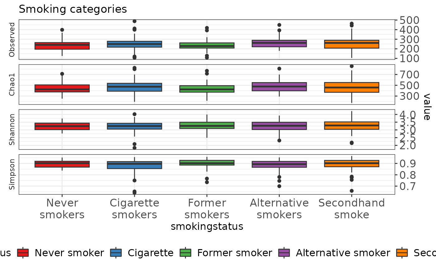
##                Df Sum Sq Mean Sq F value Pr(>F)
## smokingstatus   4   0.09 0.02162   0.168  0.954
## Residuals 254 32.62 0.12841## Df Sum Sq Mean Sq F value Pr(>F)
## smokingstatus 4 34597 8649 2.12 0.0788 .
## Residuals 254 1036314 4080
## ---
## Signif. codes: 0 '***' 0.001 '**' 0.01 '*' 0.05 '.' 0.1 ' ' 1## Df Sum Sq Mean Sq F value Pr(>F)
## smokingstatus 4 74507 18627 1.33 0.259
## Residuals 254 3556471 14002Serum cotinine vs Smoking status
ggplot(metadata, aes(smokingstatus, COTININE, fill = smokingstatus)) +
  stat_boxplot() +
  scale_fill_manual(values = scale_palette) +
  theme_bw() +
  scale_x_discrete(labels = c("Never\nsmokers","Cigarette\nsmokers", "Former\nsmokers","Alternative\nsmokers","Secondhand\nsmoke")) +
  xlab('Reported smoking status') +
  ylab('Serum Cotinine (ng/ml)') +
  guides(fill = FALSE) +
  theme(strip.background = element_rect(colour = "transparent", fill = "transparent"),
        strip.text.y = element_text(angle = 180),
        axis.text = element_text(size = 12),
        axis.title = element_text(size = 12),
        legend.text = element_text(size=12),
        legend.title = element_text(size=12),
        legend.position = 'bottom')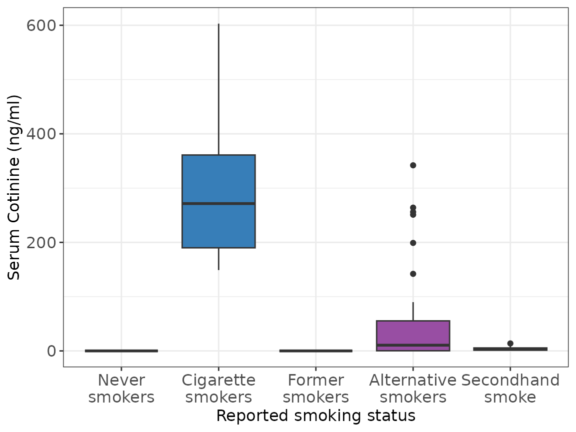
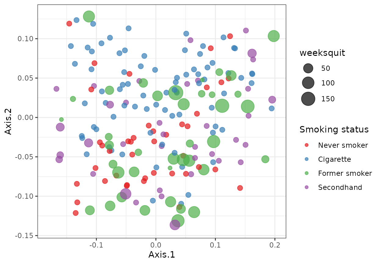
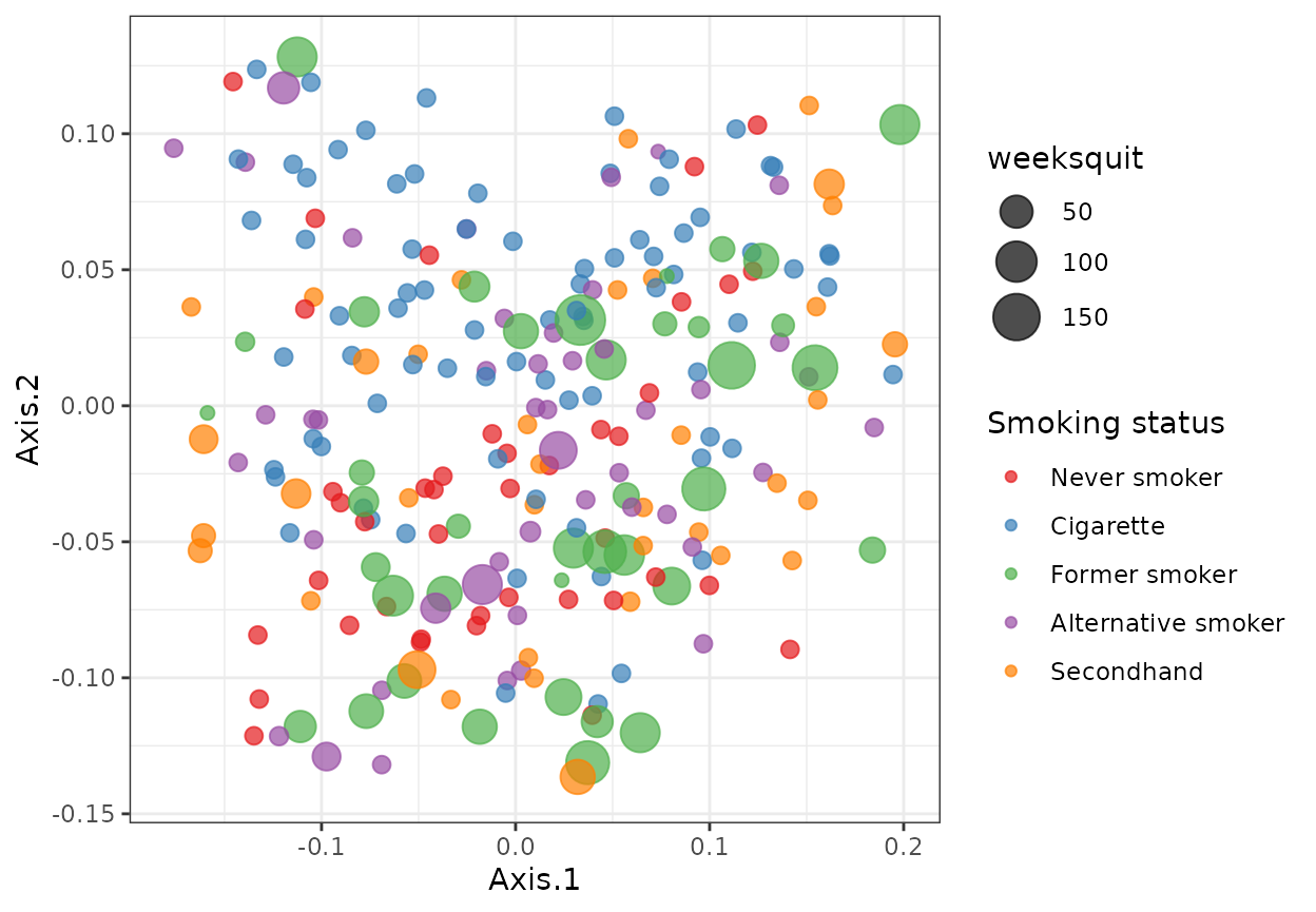
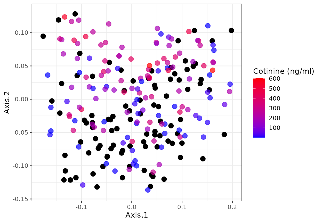
Beta Diversity
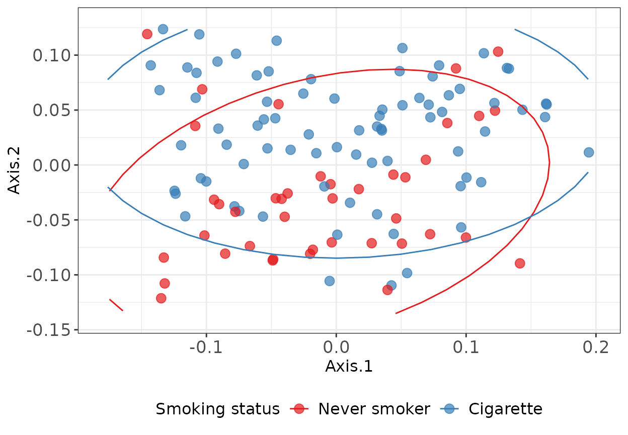

Discrete serum blood Cotinine levels
Test group with PERMANOVA (adonis, vegan package)
| contrast | r2 | pvalue |
|---|---|---|
| Never smoker vs Cigarette | 0.0561145 | 0.001 |
| Cigarette vs Former smoker | 0.0438469 | 0.001 |
| Cigarette vs Alternative smoker | 0.0311016 | 0.003 |
| Cigarette vs Secondhand | 0.0362160 | 0.003 |
| Never smoker vs Secondhand | 0.0275724 | 0.067 |
| Never smoker vs Former smoker | 0.0185099 | 0.162 |
| Former smoker vs Alternative smoker | 0.0144061 | 0.261 |
| Former smoker vs Secondhand | 0.0133631 | 0.345 |
| Alternative smoker vs Secondhand | 0.0110604 | 0.399 |
| Never smoker vs Alternative smoker | 0.0091786 | 0.527 |
## Permutation test for adonis under reduced model
## Terms added sequentially (first to last)
## Permutation: free
## Number of permutations: 999
##
## vegan::adonis2(formula = distwu_2cat ~ COTININE, data = metadata_2cat)
##           Df SumOfSqs      R2      F Pr(>F)
## COTININE   1  0.03230 0.04892 6.5318  0.001 ***
## Residual 127  0.62801 0.95108
## Total    128  0.66031 1.00000
## ---
## Signif. codes:  0 '***' 0.001 '**' 0.01 '*' 0.05 '.' 0.1 ' ' 1
Three categories
## Permutation test for adonis under reduced model
## Terms added sequentially (first to last)
## Permutation: free
## Number of permutations: 999
##
## vegan::adonis2(formula = distwu_3cat ~ smokingstatus + RACE + GENDER + AGEGRP4C + SR_ACTIVE + EDU3CAT + DBTS_NEW, data = metadata_3cat)
##                Df SumOfSqs      R2      F Pr(>F)
## smokingstatus   2  0.15260 0.05658 5.2042  0.001 ***
## RACE            4  0.08632 0.03201 1.4720  0.106
## GENDER          1  0.02643 0.00980 1.8028  0.111
## AGEGRP4C        1  0.03650 0.01353 2.4893  0.039 *
## SR_ACTIVE       2  0.03077 0.01141 1.0495  0.378
## EDU3CAT         2  0.03520 0.01305 1.2003  0.274
## DBTS_NEW        1  0.01291 0.00479 0.8804  0.496
## Residual      158  2.31644 0.85884
## Total         171  2.69717 1.00000
## ---
## Signif. codes:  0 '***' 0.001 '**' 0.01 '*' 0.05 '.' 0.1 ' ' 1
All categories
## Permutation test for adonis under reduced model
## Terms added sequentially (first to last)
## Permutation: free
## Number of permutations: 999
##
## vegan::adonis2(formula = distwu ~ smokingstatus, data = metadata)
##                Df SumOfSqs     R2      F Pr(>F)
## smokingstatus   4   0.2913 0.0488 3.2575  0.001 ***
## Residual      254   5.6793 0.9512
## Total         258   5.9707 1.0000
## ---
## Signif. codes:  0 '***' 0.001 '**' 0.01 '*' 0.05 '.' 0.1 ' ' 1
Differential analysis
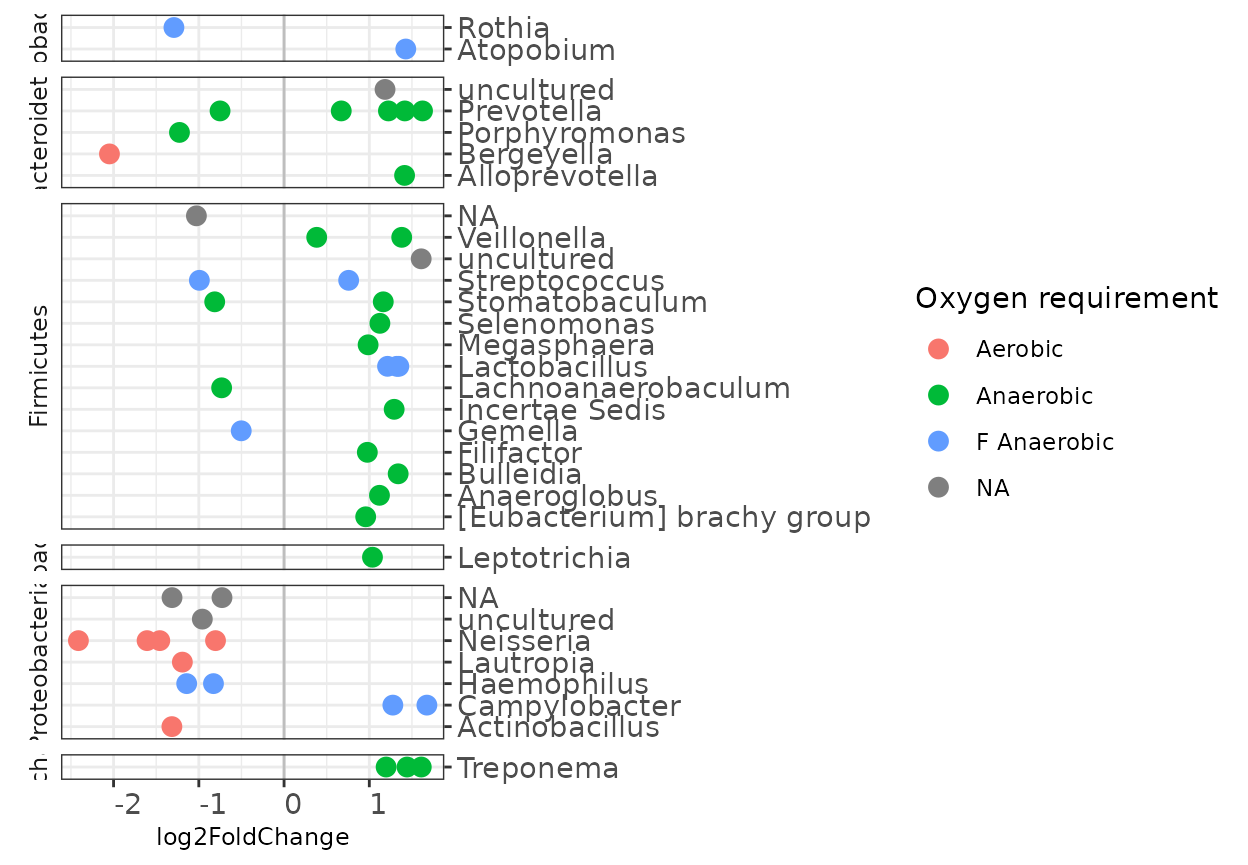


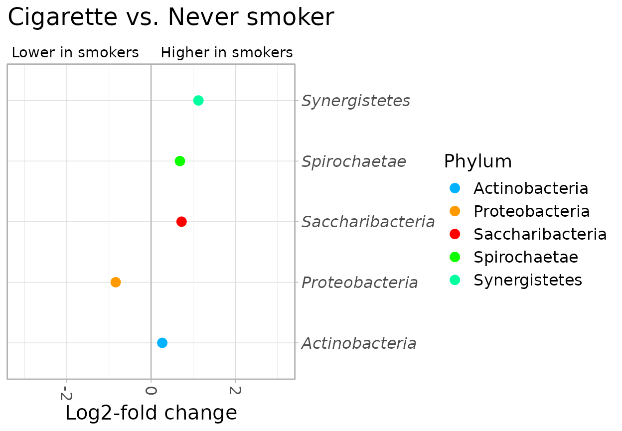
Cigarette smoker vs Never smoker: crude phylum level

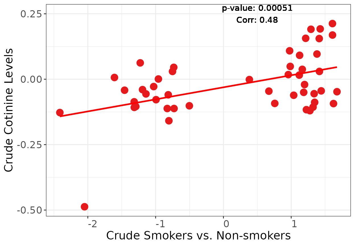
Secondhand vs Cigarette/Never: only significant OTUs
A function for merging smoking and cotinine edgeR results:
mergeResults <- function(obj.smoking, obj.cotinine) {
  intersect.filters <-
    intersect(rownames(obj.smoking), rownames(obj.cotinine))
  intersect.filters <- sort(intersect.filters)
  obj.smoking <- obj.smoking[intersect.filters, ]
  obj.cotinine <- obj.cotinine[intersect.filters, ]
  stopifnot(all.equal(rownames(obj.smoking), rownames(obj.cotinine)))
  ##
  res <-
    data.frame(
      logFC_smoking = obj.smoking$table$logFC,
      logFC_cotinine = obj.cotinine$table$logFC,
      FDR_smoking = obj.smoking$table$FDR,
      FDR_cotinine = obj.cotinine$table$FDR,
      OTU = rownames(obj.smoking$table)
    )
  res <- cbind(res, obj.smoking[, c("Phylum", "Class", "Order", "Family", "Genus", "Species")])
  return(res)
}
And a plotting function:
plotSmokingcotinineComparison <-
  function(obj.smoking,
           obj.cotinine,
           labtext = "Crude",
           FDRcutoff = 1) {
    dataset <- mergeResults(obj.smoking, obj.cotinine)
    dataset <- dataset[dataset$FDR_smoking < FDRcutoff,]
    corr.result <- with(dataset,
                        cor.test(logFC_smoking, logFC_cotinine))
    p <- ggplot(dataset) +
      theme_bw() +
      xlab(paste(labtext, "Smokers vs. Non-smokers")) +
      ylab(paste(labtext, "Cotinine Levels (ng/ml)")) +
      geom_text(aes(1,-0.3, label = sprintf(
        "p-value: %s\ncor: %s \nFDR<0.05: %s",
        signif(corr.result$p.value, 2),
        signif(corr.result$estimate, 2),
        sum(dataset$FDR_smoking < 0.05)
      )), size = 5) +
      geom_point(aes(logFC_smoking, logFC_cotinine, color = FDR_smoking <= 0.05),
                 size = 3) +
      scale_colour_manual(values = setNames(c('black', 'grey'), c(TRUE, FALSE)), guide =
                            FALSE) +
      geom_smooth(
        aes(logFC_smoking, logFC_cotinine),
        method = lm,
        se = FALSE,
        color = "red"
      ) +
      theme(
        axis.text = element_text(
          hjust = 0,
          vjust = 0.5,
          size = 13
        ),
        strip.text = element_text(size = 13),
        axis.title = element_text(size = 15)
      )
    return(p)
  }
Two thresholds for serum cotinine:
NYC_HANES.secondhand.original <- subset_samples(NYC_HANES, smokingstatus %in% c("Secondhand"))
NYC_HANES.secondhand.strict <- subset_samples(NYC_HANES.secondhand.original, COTININE < 10)
sort(sample_data(NYC_HANES.secondhand.original)$COTININE)
## [1] 1.0022 1.0394 1.0418 1.0715 1.0915 1.2015 1.2282 1.2718 1.3822
## [10] 1.3822 1.4094 1.5315 1.6918 2.0094 2.5994 2.6759 2.8020 2.9394
## [19] 2.9720 3.0459 3.1082 3.1722 3.4715 3.8394 4.3418 4.5294 4.5394
## [28] 4.7522 5.7220 6.3118 7.1315 7.7382 9.1118 9.6415 10.2922 10.6920
## [37] 10.7915 13.7894
summary(sample_data(NYC_HANES.secondhand.original)$COTININE > 10)## Mode FALSE TRUE
## logical 34 4Number of OTUs with FDR < 0.05 and total that passed non-specific screens in both analysis:
summary(edger.smoker_secondhand_crude$FDR_smoking < 0.05)## Mode FALSE TRUE
## logical 93 28
# note that the different total number for strict cotinine cutoff is
# due to non-specific filtering in edgeR
summary(edger.smoker_secondhand_crude.strict$FDR_smoking < 0.05)
## Mode FALSE TRUE
## logical 87 27
corarray <- array(dim=c(2, 2, 2), dimnames=list(secondhand=c("cot14", "cot10"),
                                                counfounding=c("crude", "adjusted"),
                                                FDRcutoff=c("no", "yes")))
parray <- array(dim=c(2, 2, 2), dimnames=list(secondhand=c("cot14", "cot10"),
                                                counfounding=c("crude", "adjusted"),
                                                FDRcutoff=c("no", "yes")))
Correlation between crude smoking and cotinine coefficients, all OTUs:
corr <- with(edger.smoker_secondhand_crude,
     cor.test(logFC_smoking, logFC_cotinine))
parray["cot14", "crude", "no"] <- corr$p.value
corarray["cot14", "crude", "no"] <- corr$estimate
Strict definition of second-hand smoke:
corr <- with(edger.smoker_secondhand_crude.strict,
     cor.test(logFC_smoking, logFC_cotinine))
parray["cot10", "crude", "no"] <- corr$p.value
corarray["cot10", "crude", "no"] <- corr$estimate
Correlation between crude smoking and cotinine coefficients, FDR < 0.05 in smoking:
corr <- with(filter(edger.smoker_secondhand_crude, FDR_smoking < 0.05),
  cor.test(logFC_smoking, logFC_cotinine))
corarray["cot10", "crude", "yes"] <- corr$p.value
parray["cot10", "crude", "yes"] <- corr$estimate
All OTUs, black for FDR < 0.05 on smoking coefficients, grey for FDR >= 0.05
p <-
  plotSmokingcotinineComparison(dasmoking.crude,
                                dacot.crude,
                                labtext = "Crude",
                                FDR = 1)
p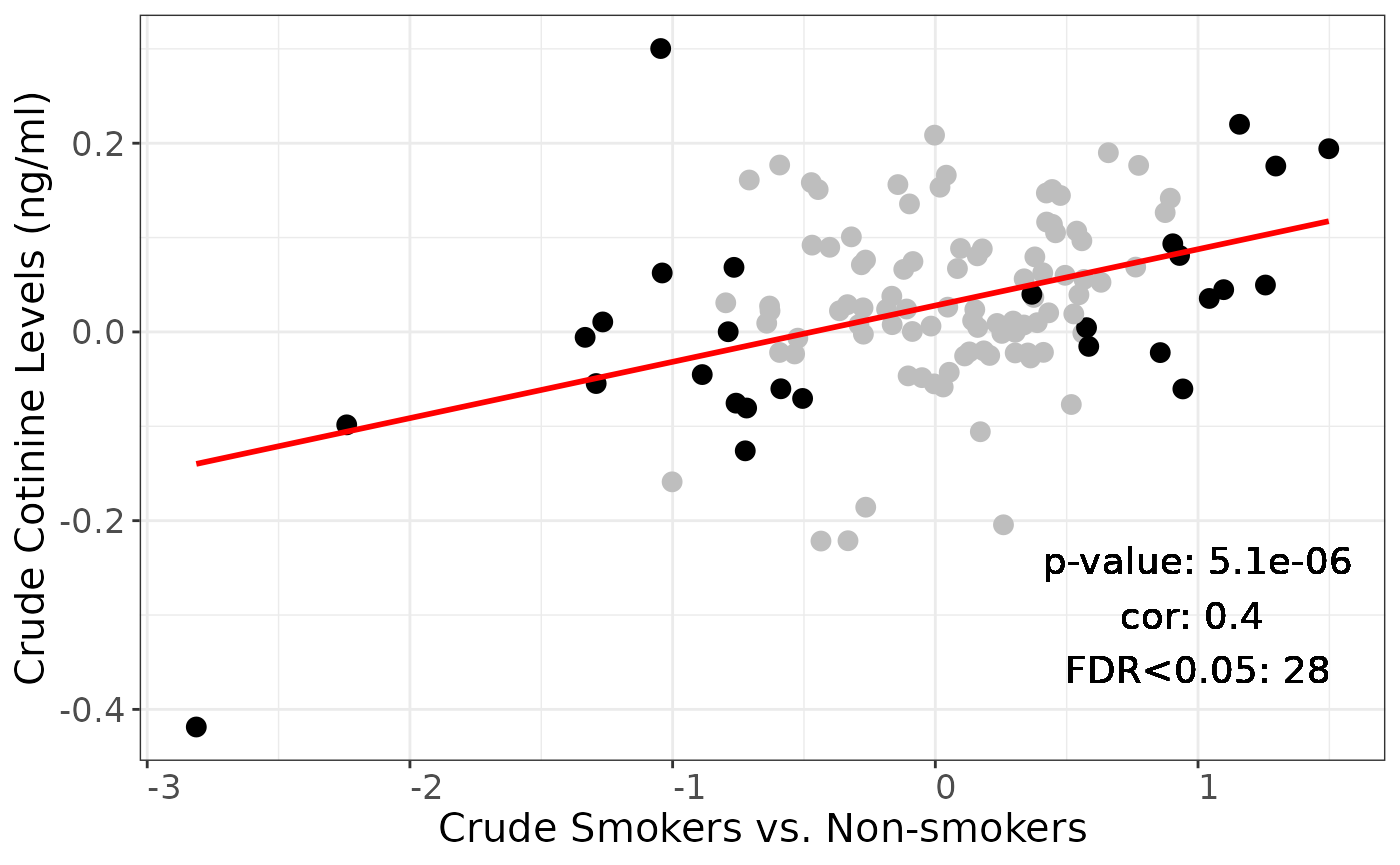
Repeat, using the strict definition of second-hand smokers (cotinine < 10)
p <-
  plotSmokingcotinineComparison(dasmoking.crude,
                                dacot.crude.strict,
                                labtext = "Crude",
                                FDR = 1)
p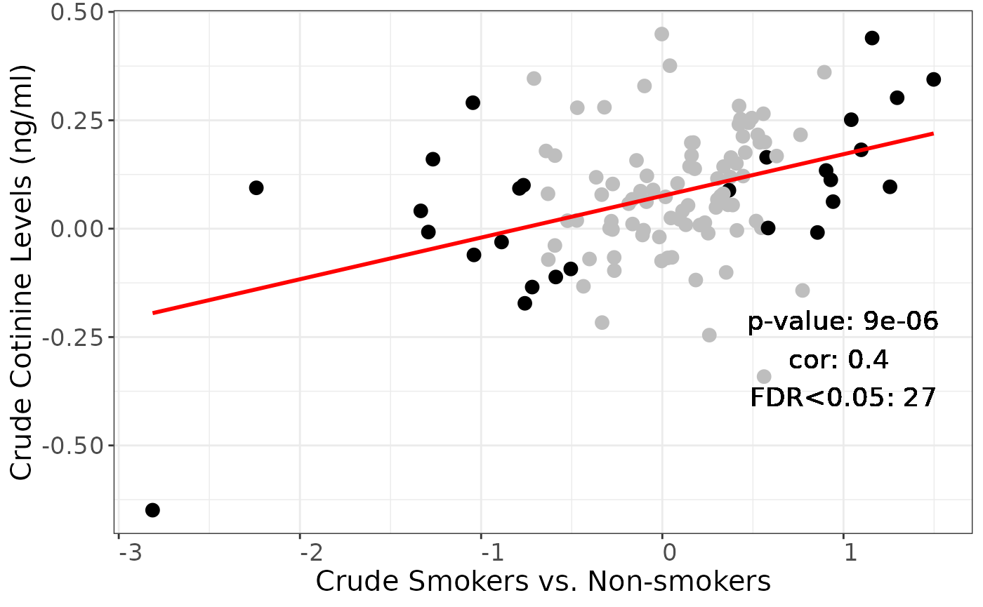
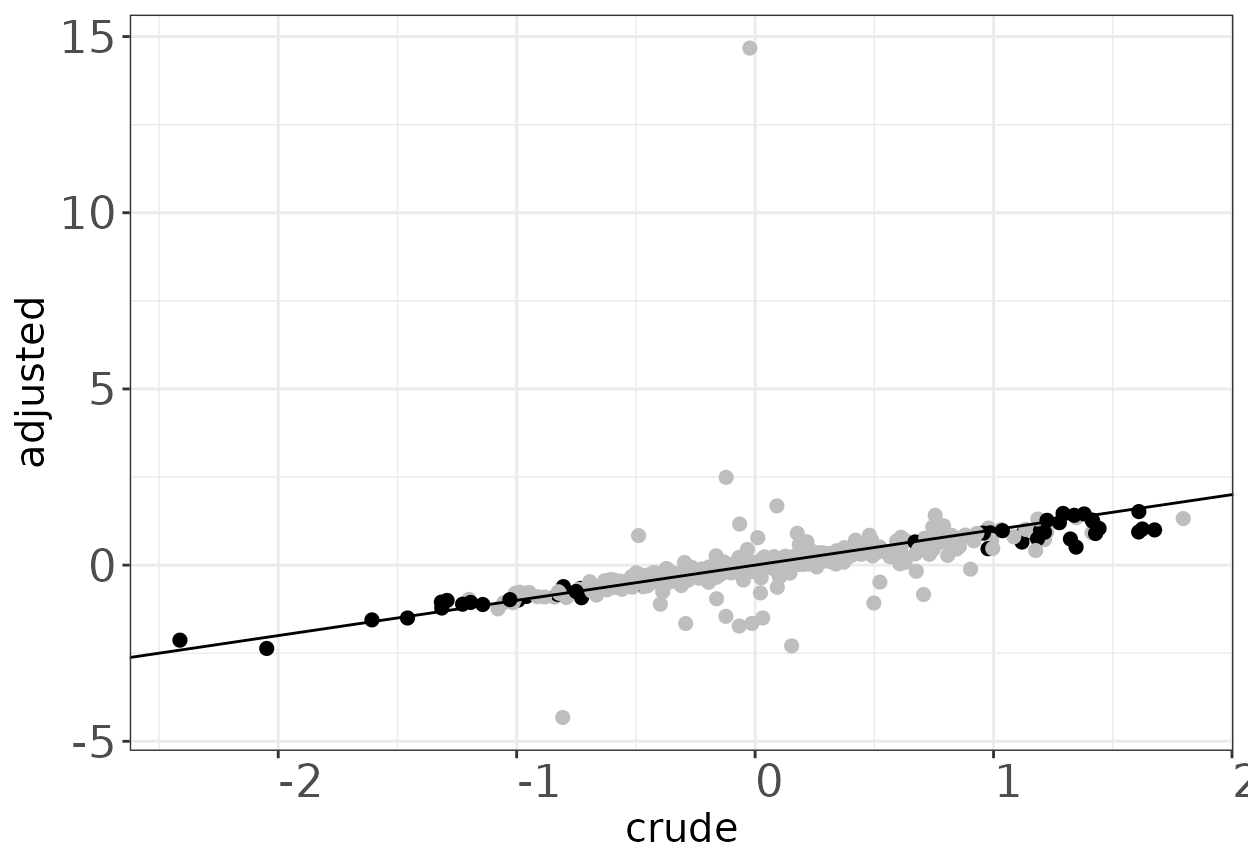
Adjusted Secondhand vs Adjusted Cigarette/Never: only significant OTUs
Number of differentially abundant OTUs, and total
nrow(edger.smoker_secondhand_adjusted)## [1] 121
summary(edger.smoker_secondhand_adjusted$logFC_smoking < 0.05)## Mode FALSE TRUE
## logical 63 58
summary(edger.smoker_secondhand_adjusted$logFC_cotinine < 0.05)## Mode FALSE TRUE
## logical 38 83Correlation between adjusted smoking and cotinine coefficients, all OTUs:
corr <- with(edger.smoker_secondhand_adjusted,
     cor.test(logFC_smoking, logFC_cotinine))
parray["cot14", "adjusted", "no"] <- corr$p.value
corarray["cot14", "adjusted", "no"] <- corr$estimate
As above, using strict serum cotinine cutoff (<10)
corr <- with(edger.smoker_secondhand_adjusted.strict,
     cor.test(logFC_smoking, logFC_cotinine))
parray["cot10", "adjusted", "no"] <- corr$p.value
corarray["cot10", "adjusted", "no"] <- corr$estimate
Correlation between adjusted smoking and cotinine coefficients, FDR < 0.05 in smoking:
with(filter(edger.smoker_secondhand_adjusted, FDR_smoking < 0.05),
  cor.test(logFC_smoking, logFC_cotinine))
##
## Pearson's product-moment correlation
##
## data: logFC_smoking and logFC_cotinine
## t = 3.8131, df = 17, p-value = 0.001391
## alternative hypothesis: true correlation is not equal to 0
## 95 percent confidence interval:
## 0.3249855 0.8660843
## sample estimates:
## cor
## 0.6789709
parray["cot14", "adjusted", "yes"] <- corr$p.value
corarray["cot14", "adjusted", "yes"] <- corr$estimate
Sensitivity analysis:
round(corarray, 2)## , , FDRcutoff = no
##
## counfounding
## secondhand crude adjusted
## cot14 0.4 0.28
## cot10 0.4 0.34
##
## , , FDRcutoff = yes
##
## counfounding
## secondhand crude adjusted
## cot14 NA 0.34
## cot10 0 NA
signif(parray, 1)## , , FDRcutoff = no
##
## counfounding
## secondhand crude adjusted
## cot14 5e-06 2e-03
## cot10 9e-06 3e-04
##
## , , FDRcutoff = yes
##
## counfounding
## secondhand crude adjusted
## cot14 NA 3e-04
## cot10 0.6 NA
p <-
  plotSmokingcotinineComparison(
    obj.smoking = dasmoking.adjusted,
    obj.cotinine = dacot.adjusted,
    labtext = "Adjusted",
    FDRcutoff = 1
  )
p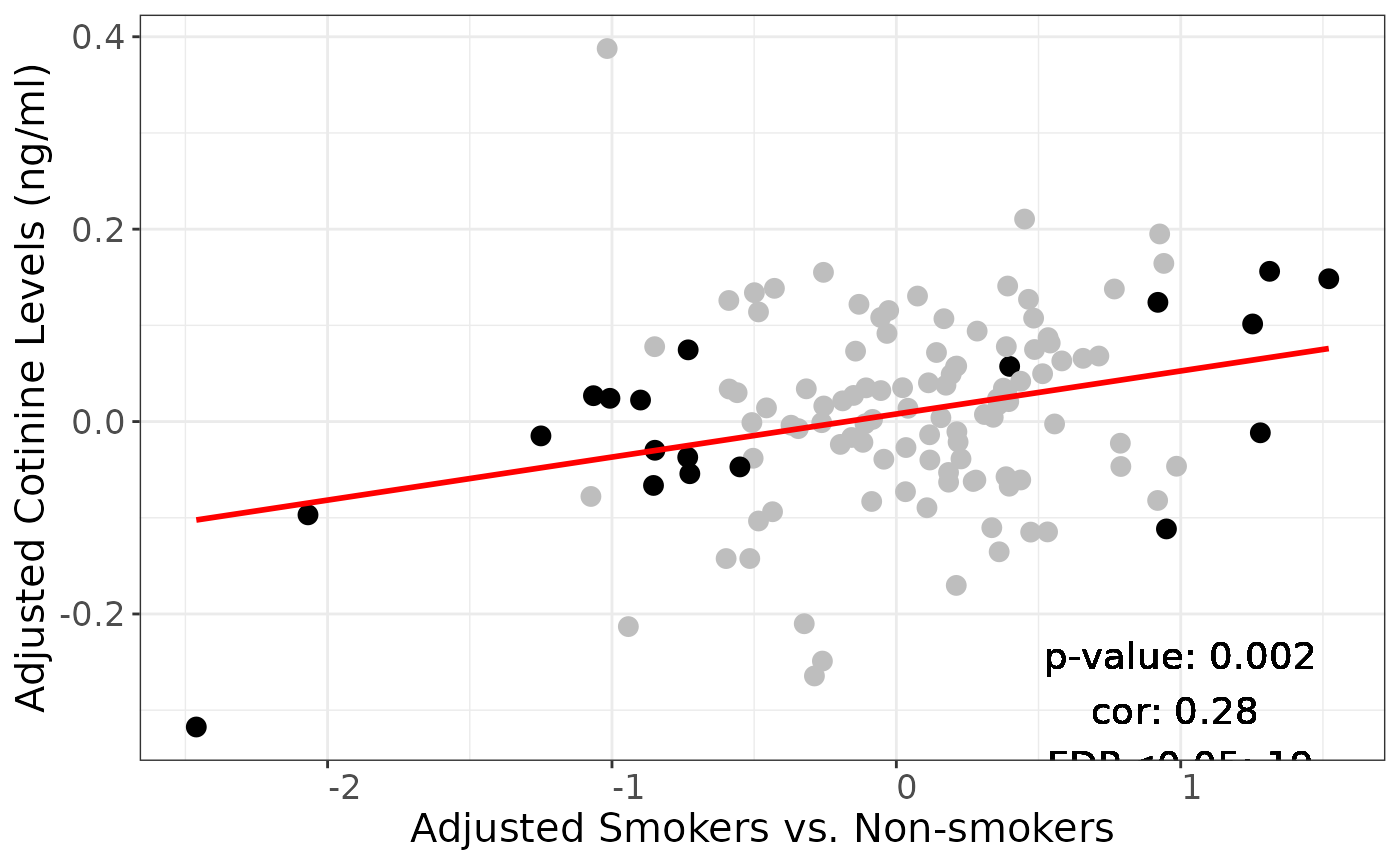
Repeat, using the strict definition of second-hand smokers (cotinine < 10)
p <-
  plotSmokingcotinineComparison(
    obj.smoking = dasmoking.adjusted,
    obj.cotinine = dacot.adjusted.strict,
    labtext = "Adjusted",
    FDRcutoff = 1
  )
p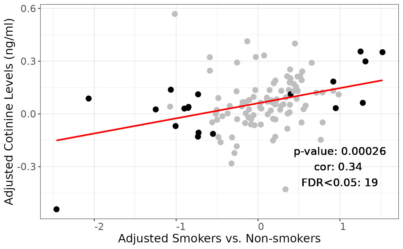
Write supplemental file
stopifnot(all.equal(rownames(edger.smoker_secondhand_adjusted),
                    rownames(edger.smoker_secondhand_crude)))
crude <- edger.smoker_secondhand_crude[, 1:4]
adjusted <- edger.smoker_secondhand_adjusted[, 1:4]
colnames(crude) <- paste0(colnames(crude), "_crude")
colnames(adjusted) <- paste0(colnames(adjusted), "_adjusted")
sfile <- cbind(edger.smoker_secondhand_crude[, -1:-4], crude, adjusted)
readr::write_excel_csv(sfile, path="SupplementalFile1.csv")
Analysis on biosis of bacteria
Odds ratio smokers vs never smokers
## $tab
##
##                      Enriched in smokers        p0 Depleted in smokers
##   OTU is aerobic                      23 0.0362776                  55
##   OTU is not aerobic                 611 0.9637224                 457
##
##                             p1 oddsratio     lower     upper      p.value
##   OTU is aerobic     0.1074219 1.0000000        NA        NA           NA
##   OTU is not aerobic 0.8925781 0.3127808 0.1894164 0.5164911 2.682452e-06
##
## $measure
## [1] "wald"
##
## $conf.level
## [1] 0.95
##
## $pvalue
## [1] "fisher.exact"
## $tab
##
## Enriched in smokers p0 Depleted in smokers
## OTU is anaerobic 407 0.6419558 266
## OTU is not anaerobic 227 0.3580442 246
##
## p1 oddsratio lower upper p.value
## OTU is anaerobic 0.5195312 1.000000 NA NA NA
## OTU is not anaerobic 0.4804688 1.658143 1.307573 2.102704 3.107853e-05
##
## $measure
## [1] "wald"
##
## $conf.level
## [1] 0.95
##
## $pvalue
## [1] "fisher.exact"## $tab
##
## Enriched in smokers p0 Depleted in smokers
## OTU is F Anaerobic 204 0.3217666 191
## OTU is not F Anaerobic 430 0.6782334 321
##
## p1 oddsratio lower upper p.value
## OTU is F Anaerobic 0.3730469 1.0000000 NA NA NA
## OTU is not F Anaerobic 0.6269531 0.7973213 0.624298 1.018298 0.07029177
##
## $measure
## [1] "wald"
##
## $conf.level
## [1] 0.95
##
## $pvalue
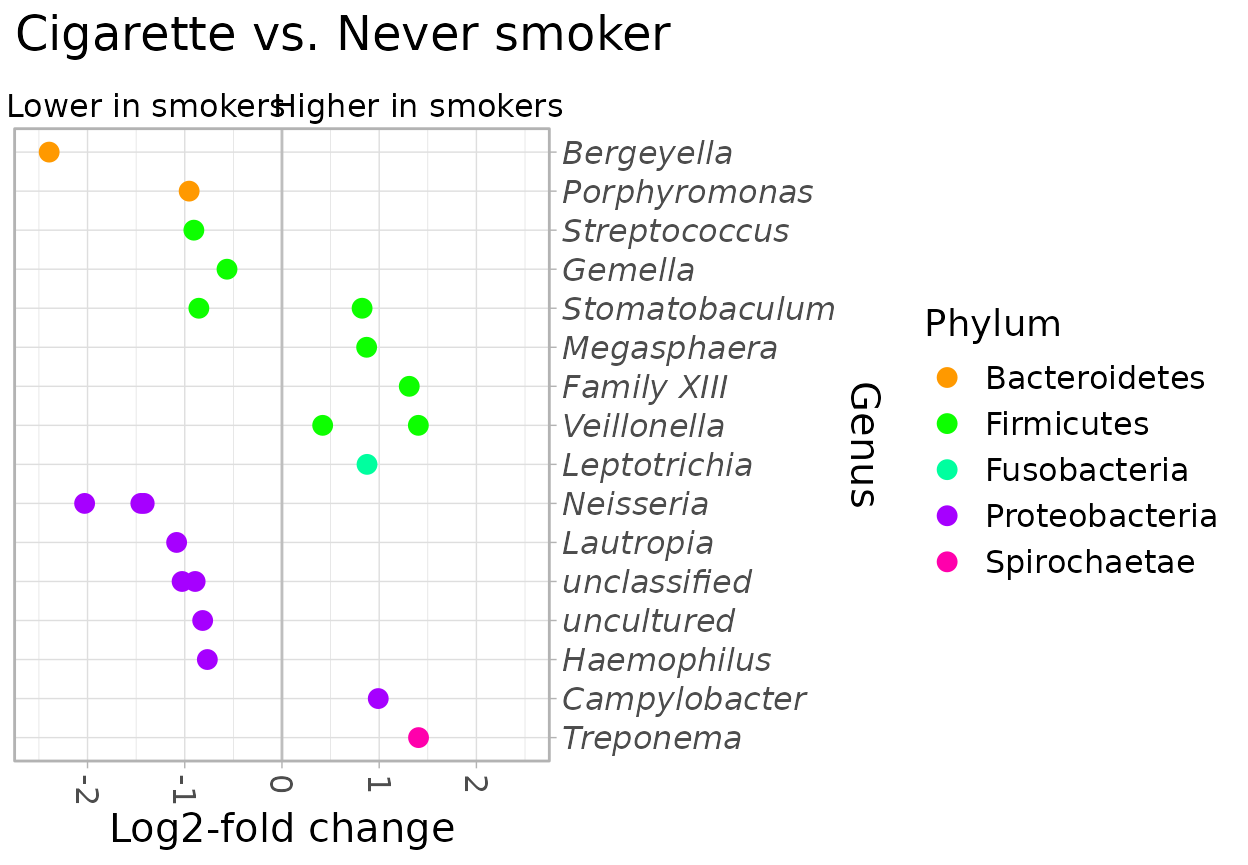
## [1] "fisher.exact"Cigarette smokers vs Never smokers
GSEA
## DataFrame with 2 rows and 4 columns
##      GENE.SET        ES       NES      PVAL
##   <character> <numeric> <numeric> <numeric>
## 1        aero    -0.545     -1.90   0.00378
## 2        fana    -0.254     -1.08   0.36200
ORA
## 100 permutations completed
## 200 permutations completed
## 300 permutations completed
## 400 permutations completed
## 500 permutations completed
## 600 permutations completed
## 700 permutations completed
## 800 permutations completed
## 900 permutations completed
## 1000 permutations completed
## DataFrame with 2 rows and 4 columns
## GENE.SET GLOB.STAT NGLOB.STAT PVAL
## <character> <numeric> <numeric> <numeric>
## 1 aero 13 0.167 0.001
## 2 fana 17 0.043 0.999Secondhand smokers
GSEA
## DataFrame with 2 rows and 4 columns
##      GENE.SET        ES       NES      PVAL
##   <character> <numeric> <numeric> <numeric>
## 1        fana    -0.288     -1.17     0.233
## 2        aero    -0.337     -1.21     0.237
ORA
## 100 permutations completed
## 200 permutations completed
## 300 permutations completed
## 400 permutations completed
## 500 permutations completed
## 600 permutations completed
## 700 permutations completed
## 800 permutations completed
## 900 permutations completed
## 1000 permutations completed
## DataFrame with 2 rows and 4 columns
## GENE.SET GLOB.STAT NGLOB.STAT PVAL
## <character> <numeric> <numeric> <numeric>
## 1 fana 1 0.00253 0.001
## 2 aero 0 0.00000 0.193Continuous cotinine
GSVA continuous cotinine on secondhand smokers
## Estimating GSVA scores for 3 gene sets.
## Estimating ECDFs with Gaussian kernels
##   |                                                                              |                                                                      |   0%  |                                                                              |=======================                                               |  33%  |                                                                              |===============================================                       |  67%  |                                                                              |======================================================================| 100%
## logFC AveExpr t P.Value adj.P.Val B
## aero 0.0049390950 0.063396833 0.8947032 0.3756454 0.6151923 -7.392942
## anae 0.0029017486 -0.003614764 0.8313163 0.4101282 0.6151923 -7.447853
## fana 0.0007153343 0.034927979 0.1784040 0.8591962 0.8591962 -7.781513GSVA continuous cotinine on cigarette vs never smokers
## Estimating GSVA scores for 3 gene sets.
## Estimating ECDFs with Gaussian kernels
##   |                                                                              |                                                                      |   0%  |                                                                              |=======================                                               |  33%  |                                                                              |===============================================                       |  67%  |                                                                              |======================================================================| 100%
## logFC AveExpr t P.Value adj.P.Val B
## anae 9.312388e-05 0.01061843 2.635005 0.009409142 0.02519808 -8.951131
## fana -1.031180e-04 -0.02637825 -2.421534 0.016798721 0.02519808 -9.469995
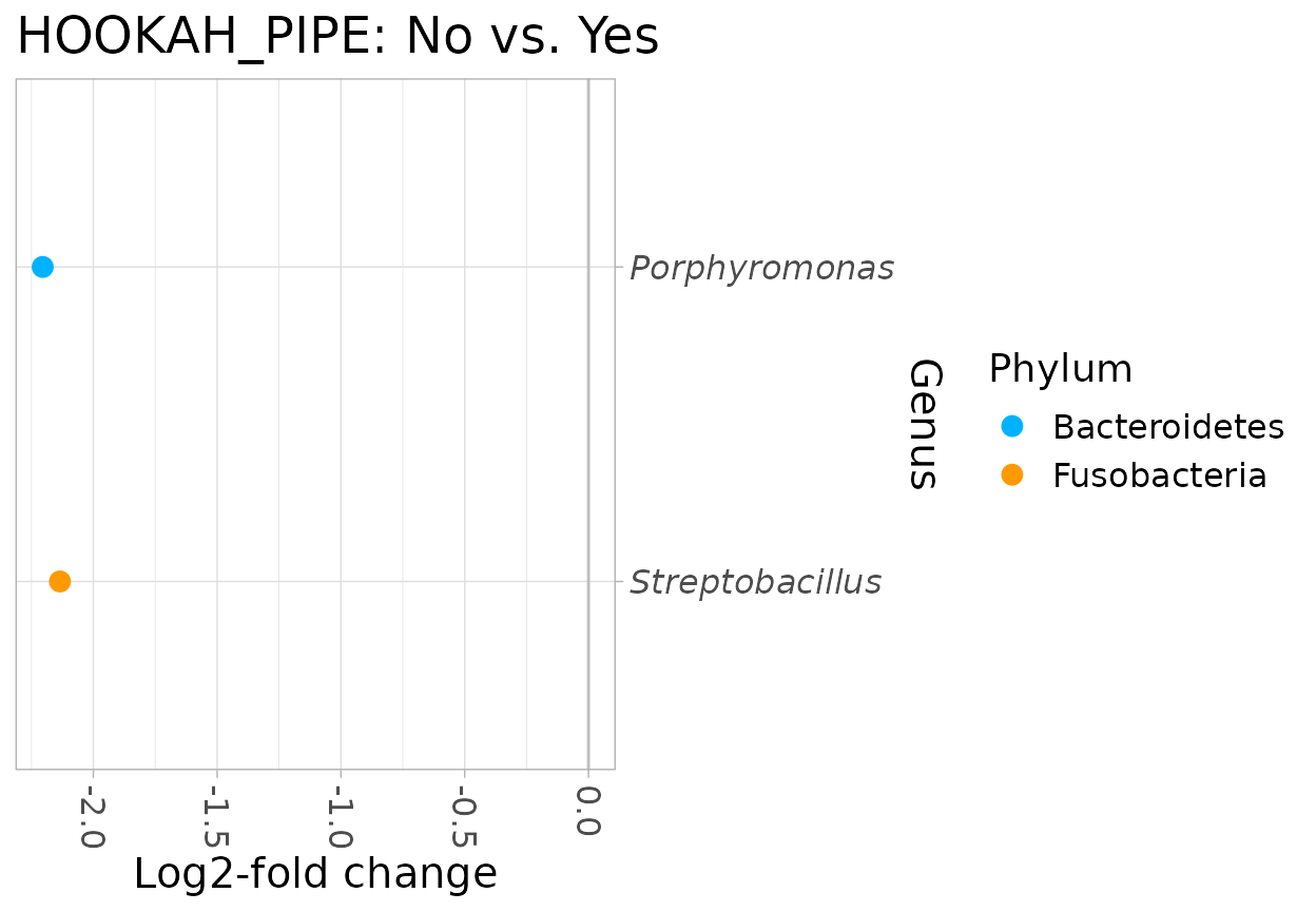
## aero 9.331210e-05 0.10299623 1.397472 0.164590432 0.16459043 -11.384173Hookah smokers vs Never smokers
E-cigarette smokers vs Never smokers
Cigar/cigarillos smokers vs Never smokers
GSEA
## DataFrame with 2 rows and 4 columns
##      GENE.SET        ES       NES      PVAL
##   <character> <numeric> <numeric> <numeric>
## 1        aero    -0.367    -1.280     0.146
## 2        fana    -0.166    -0.728     0.879
ORA
## DataFrame with 2 rows and 4 columns
##      GENE.SET  NR.GENES NR.SIG.GENES      PVAL
##   <character> <numeric>    <numeric> <numeric>
## 1        fana       395            3     0.582
## 2 aero 78 0 1.000## R version 4.3.3 (2024-02-29)
## Platform: x86_64-pc-linux-gnu (64-bit)
## Running under: Ubuntu 22.04.4 LTS
##
## Matrix products: default
## BLAS: /usr/lib/x86_64-linux-gnu/openblas-pthread/libblas.so.3
## LAPACK: /usr/lib/x86_64-linux-gnu/openblas-pthread/libopenblasp-r0.3.20.so; LAPACK version 3.10.0
##
## locale:
## [1] LC_CTYPE=C.UTF-8 LC_NUMERIC=C LC_TIME=C.UTF-8
## [4] LC_COLLATE=C.UTF-8 LC_MONETARY=C.UTF-8 LC_MESSAGES=C.UTF-8
## [7] LC_PAPER=C.UTF-8 LC_NAME=C LC_ADDRESS=C
## [10] LC_TELEPHONE=C LC_MEASUREMENT=C.UTF-8 LC_IDENTIFICATION=C
##
## time zone: UTC
## tzcode source: system (glibc)
##
## attached base packages:
## [1] stats graphics grDevices utils datasets methods base
##
## other attached packages:
## [1] edgeR_4.0.16 limma_3.58.1 ggplot2_3.5.0
## [4] magrittr_2.0.3 dplyr_1.1.4 nychanesmicrobiome_0.1.2
## [7] lsr_0.5.2 phyloseq_1.46.0 Biobase_2.62.0
## [10] BiocGenerics_0.48.1 BiocStyle_2.30.0
##
## loaded via a namespace (and not attached):
## [1] splines_4.3.3 bitops_1.0-7
## [3] tibble_3.2.1 R.oo_1.26.0
## [5] graph_1.80.0 XML_3.99-0.16.1
## [7] lifecycle_1.0.4 doParallel_1.0.17
## [9] lattice_0.22-5 vroom_1.6.5
## [11] MASS_7.3-60.0.1 survey_4.4-2
## [13] sass_0.4.9 rmarkdown_2.26
## [15] jquerylib_0.1.4 yaml_2.3.8
## [17] DBI_1.2.2 RColorBrewer_1.1-3
## [19] ade4_1.7-22 abind_1.4-5
## [21] zlibbioc_1.48.2 Rtsne_0.17
## [23] GenomicRanges_1.54.1 purrr_1.0.2
## [25] R.utils_2.12.3 RCurl_1.98-1.14
## [27] circlize_0.4.16 labelled_2.12.0
## [29] GenomeInfoDbData_1.2.11 IRanges_2.36.0
## [31] S4Vectors_0.40.2 irlba_2.3.5.1
## [33] GSVA_1.50.5 vegan_2.6-4
## [35] microbiome_1.24.0 annotate_1.80.0
## [37] DelayedMatrixStats_1.24.0 pkgdown_2.0.8
## [39] permute_0.9-7 codetools_0.2-19
## [41] DelayedArray_0.28.0 tidyselect_1.2.1
## [43] shape_1.4.6.1 farver_2.1.1
## [45] ScaledMatrix_1.10.0 epitools_0.5-10.1
## [47] matrixStats_1.3.0 stats4_4.3.3
## [49] jsonlite_1.8.8 GetoptLong_1.0.5
## [51] multtest_2.58.0 e1071_1.7-14
## [53] survival_3.5-8 iterators_1.0.14
## [55] systemfonts_1.0.6 foreach_1.5.2
## [57] tools_4.3.3 ragg_1.3.0
## [59] Rcpp_1.0.12 glue_1.7.0
## [61] SparseArray_1.2.4 xfun_0.43
## [63] mgcv_1.9-1 DESeq2_1.42.1
## [65] MatrixGenerics_1.14.0 GenomeInfoDb_1.38.8
## [67] HDF5Array_1.30.1 withr_3.0.0
## [69] BiocManager_1.30.22 fastmap_1.1.1
## [71] mitools_2.4 rhdf5filters_1.14.1
## [73] fansi_1.0.6 SparseM_1.81
## [75] rsvd_1.0.5 digest_0.6.35
## [77] R6_2.5.1 textshaping_0.3.7
## [79] colorspace_2.1-0 RSQLite_2.3.6
## [81] R.methodsS3_1.8.2 utf8_1.2.4
## [83] tidyr_1.3.1 generics_0.1.3
## [85] data.table_1.15.4 class_7.3-22
## [87] httr_1.4.7 htmlwidgets_1.6.4
## [89] S4Arrays_1.2.1 pkgconfig_2.0.3
## [91] gtable_0.3.4 blob_1.2.4
## [93] ComplexHeatmap_2.18.0 SingleCellExperiment_1.24.0
## [95] XVector_0.42.0 htmltools_0.5.8.1
## [97] bookdown_0.39 biomformat_1.30.0
## [99] GSEABase_1.64.0 clue_0.3-65
## [101] scales_1.3.0 png_0.1-8
## [103] knitr_1.46 tzdb_0.4.0
## [105] reshape2_1.4.4 rjson_0.2.21
## [107] nlme_3.1-164 proxy_0.4-27
## [109] cachem_1.0.8 zoo_1.8-12
## [111] rhdf5_2.46.1 GlobalOptions_0.1.2
## [113] safe_3.42.0 stringr_1.5.1
## [115] parallel_4.3.3 AnnotationDbi_1.64.1
## [117] desc_1.4.3 pillar_1.9.0
## [119] grid_4.3.3 vctrs_0.6.5
## [121] BiocSingular_1.18.0 beachmat_2.18.1
## [123] xtable_1.8-4 cluster_2.1.6
## [125] Rgraphviz_2.46.0 evaluate_0.23
## [127] KEGGgraph_1.62.0 readr_2.1.5
## [129] cli_3.6.2 locfit_1.5-9.9
## [131] compiler_4.3.3 rlang_1.1.3
## [133] crayon_1.5.2 tableone_0.13.2
## [135] labeling_0.4.3 plyr_1.8.9
## [137] forcats_1.0.0 fs_1.6.3
## [139] stringi_1.8.3 BiocParallel_1.36.0
## [141] munsell_0.5.1 Biostrings_2.70.3
## [143] Matrix_1.6-5 sas7bdat_0.7
## [145] hms_1.1.3 sparseMatrixStats_1.14.0
## [147] bit64_4.0.5 Rhdf5lib_1.24.2
## [149] KEGGREST_1.42.0 statmod_1.5.0
## [151] SummarizedExperiment_1.32.0 highr_0.10
## [153] haven_2.5.4 igraph_2.0.3
## [155] memoise_2.0.1 bslib_0.7.0
## [157] bit_4.0.5 EnrichmentBrowser_2.32.0
## [159] ape_5.8