HMP16SData

Lucas Schiffer

Graduate School of Public Health and Health Policy, City University of New York, New York, NYInstitute for Implementation Science in Population Health, City University of New York, New York, NY

Rimsha Azhar

Graduate School of Public Health and Health Policy, City University of New York, New York, NYInstitute for Implementation Science in Population Health, City University of New York, New York, NY

Marcel Ramos

Graduate School of Public Health and Health Policy, City University of New York, New York, NYInstitute for Implementation Science in Population Health, City University of New York, New York, NYRoswell Park Cancer Institute, University of Buffalo, Buffalo, NY

Ludwig Geistlinger

Graduate School of Public Health and Health Policy, City University of New York, New York, NYInstitute for Implementation Science in Population Health, City University of New York, New York, NY

Levi Waldron

Graduate School of Public Health and Health Policy, City University of New York, New York, NYInstitute for Implementation Science in Population Health, City University of New York, New York, NY

May 5, 2025

Abstract

HMP16SData is a Bioconductor ExperimentData package of the Human Microbiome Project (HMP) 16S rRNA sequencing data for variable regions 1–3 and 3–5. Raw data files are provided in the package as downloaded from the HMP Data Analysis and Coordination Center. Processed data is provided as SummarizedExperiment class objects via ExperimentHub.

Publications

Schiffer, L. et al. HMP16SData: Efficient Access to the Human Microbiome Project through Bioconductor. Am. J. Epidemiol. (2019).

Griffith, J. C. & Morgan, X. C. Invited Commentary: Improving accessibility of the Human Microbiome Project data through integration with R/Bioconductor. Am. J. Epidemiol. (2019).

Waldron, L. et al. Waldron et al. Reply to “Commentary on the HMP16SData Bioconductor Package”. Am. J. Epidemiol. (2019).

Prerequisites

The following knitr options will be used in this vignette to provide the most useful and concise output.

knitr::opts_chunk$set(message = FALSE)

The following packages will be used in this vignette to provide demonstrative examples of what a user might do with HMP16SData.

library(HMP16SData)
library(phyloseq)
library(magrittr)
library(ggplot2)
library(tibble)
library(dplyr)
library(dendextend)
library(circlize)
library(ExperimentHub)
library(gridExtra)
library(cowplot)
library(readr)
library(haven)

Pipe operators from the magrittr package are used in this vignette to provide the most elegant and concise syntax. See the magrittr vignette if the syntax is unclear.

Introduction

HMP16SData is a Bioconductor ExperimentData package of the Human Microbiome Project (HMP) 16S rRNA sequencing data for variable regions 1–3 and 3–5. Raw data files are provided in the package as downloaded from the HMP Data Analysis and Coordination Center. Processed data is provided as SummarizedExperiment class objects via ExperimentHub.

HMP16SData can be installed using BiocManager as follows.

BiocManager::install("HMP16SData")

Once installed, HMP16SData provides two functions to access data – one for variable region 1–3 and another for variable region 3–5. When called, as follows, the functions will download data from an ExperimentHub Amazon S3 (Simple Storage Service) bucket over https or load data from a local cache.

V13()

## class: SummarizedExperiment 
## dim: 43140 2898 
## metadata(2): experimentData phylogeneticTree
## assays(1): 16SrRNA
## rownames(43140): OTU_97.1 OTU_97.10 ... OTU_97.9997 OTU_97.9999
## rowData names(7): CONSENSUS_LINEAGE SUPERKINGDOM ... FAMILY GENUS
## colnames(2898): 700013549 700014386 ... 700114963 700114965
## colData names(7): RSID VISITNO ... HMP_BODY_SUBSITE SRS_SAMPLE_ID

V35()

## class: SummarizedExperiment 
## dim: 45383 4743 
## metadata(2): experimentData phylogeneticTree
## assays(1): 16SrRNA
## rownames(45383): OTU_97.1 OTU_97.10 ... OTU_97.9998 OTU_97.9999
## rowData names(7): CONSENSUS_LINEAGE SUPERKINGDOM ... FAMILY GENUS
## colnames(4743): 700013549 700014386 ... 700114717 700114750
## colData names(7): RSID VISITNO ... HMP_BODY_SUBSITE SRS_SAMPLE_ID

The two data sets are represented as SummarizedExperiment objects, a standard Bioconductor class that is amenable to subsetting and analysis. To maintain brevity, details of the SummarizedExperiment class are not outlined here but the SummarizedExperiment package provides an excellent vignette.

Features

Frequency Table Generation

Sometimes it is desirable to provide a quick summary of key demographic variables and to make the process easier HMP16SData provides a function, table_one, to do so. It returns a data.frame or a list of data.frame objects that have been transformed to make a publication ready table.

V13() %>%
    table_one() %>%
    head()

##           Visit Number    Sex                                  Run Center
## 700013549          One Female                  Baylor College of Medicine
## 700014386          One   Male Baylor College of Medicine, Broad Institute
## 700014403          One   Male Baylor College of Medicine, Broad Institute
## 700014409          One   Male Baylor College of Medicine, Broad Institute
## 700014412          One   Male Baylor College of Medicine, Broad Institute
## 700014415          One   Male Baylor College of Medicine, Broad Institute
##                    HMP Body Site HMP Body Subsite
## 700013549 Gastrointestinal Tract            Stool
## 700014386 Gastrointestinal Tract            Stool
## 700014403                   Oral           Saliva
## 700014409                   Oral    Tongue Dorsum
## 700014412                   Oral      Hard Palate
## 700014415                   Oral    Buccal Mucosa

If a list is passed to table_one, its elements must be named so that the named elements can be used by the kable_one function. The kable_one function will produce an HTML table for vignettes such as the one shown below.

list(V13 = V13(), V35 = V35()) %>%
    table_one() %>%
    kable_one()

	V13		V35
	N	%	N	%
Visit Number
One	1,642	56.66	2,822	59.50
Two	1,244	42.93	1,897	40.00
Three	12	0.41	24	0.51
Sex
Female	1,521	52.48	2,188	46.13
Male	1,377	47.52	2,555	53.87
Run Center
Genome Sequencing Center at Washington University	1,717	59.25	1,539	32.45
J. Craig Venter Institute	506	17.46	1,009	21.27
Broad Institute	0	0.00	1,078	22.73
Baylor College of Medicine	289	9.97	696	14.67
J. Craig Venter Institute, Genome Sequencing Center at Washington University	97	3.35	93	1.96
Baylor College of Medicine, Genome Sequencing Center at Washington University	91	3.14	90	1.90
Baylor College of Medicine, Broad Institute	76	2.62	103	2.17
J. Craig Venter Institute, Broad Institute	86	2.97	75	1.58
Baylor College of Medicine, J. Craig Venter Institute	15	0.52	40	0.84
Broad Institute, Baylor College of Medicine	13	0.45	13	0.27
Genome Sequencing Center at Washington University, Baylor College of Medicine	6	0.21	6	0.13
Genome Sequencing Center at Washington University, J. Craig Venter Institute	1	0.03	1	0.02
Missing	1	0.03	0	0.00
HMP Body Site
Oral	1,622	55.97	2,774	58.49
Skin	664	22.91	990	20.87
Urogenital Tract	264	9.11	391	8.24
Gastrointestinal Tract	187	6.45	319	6.73
Airways	161	5.56	269	5.67
HMP Body Subsite
Tongue Dorsum	190	6.56	316	6.66
Stool	187	6.45	319	6.73
Supragingival Plaque	189	6.52	313	6.60
Right Retroauricular Crease	187	6.45	297	6.26
Attached Keratinized Gingiva	181	6.25	313	6.60
Left Retroauricular Crease	186	6.42	285	6.01
Buccal Mucosa	183	6.31	312	6.58
Palatine Tonsils	186	6.42	312	6.58
Subgingival Plaque	183	6.31	309	6.51
Throat	170	5.87	307	6.47
Hard Palate	178	6.14	302	6.37
Saliva	162	5.59	290	6.11
Anterior Nares	161	5.56	269	5.67
Right Antecubital Fossa	146	5.04	207	4.36
Left Antecubital Fossa	145	5.00	201	4.24
Mid Vagina	89	3.07	133	2.80
Posterior Fornix	88	3.04	133	2.80
Vaginal Introitus	87	3.00	125	2.64

Straightforward Subsetting

The SummarizedExperiment container provides for straightforward subsetting by data or metadata variables using either the subset function or [ methods – see the SummarizedExperiment vignette for additional details. Shown below, the variable region 3–5 data set is subset to include only stool samples.

V35_stool <-
    V35() %>%
    subset(select = HMP_BODY_SUBSITE == "Stool")

V35_stool

## class: SummarizedExperiment 
## dim: 45383 319 
## metadata(2): experimentData phylogeneticTree
## assays(1): 16SrRNA
## rownames(45383): OTU_97.1 OTU_97.10 ... OTU_97.9998 OTU_97.9999
## rowData names(7): CONSENSUS_LINEAGE SUPERKINGDOM ... FAMILY GENUS
## colnames(319): 700013549 700014386 ... 700114717 700114750
## colData names(7): RSID VISITNO ... HMP_BODY_SUBSITE SRS_SAMPLE_ID

HMP Controlled-Access Participant Data

Most participant data from the HMP study is controlled through the National Center for Biotechnology Information (NCBI) database of Genotypes and Phenotypes (dbGaP). HMP16SData provides a data dictionary translated from dbGaP XML files for the seven different controlled-access data tables related to the HMP. See ?HMP16SData::dictionary for details of these source data tables, and View(dictionary) to view the complete data dictionary. Several steps are required to access the data tables, but the process is greatly simplified by HMP16SData.

Apply for dbGaP Access

You must make a controlled-access application through https://dbgap.ncbi.nlm.nih.gov for:

HMP Core Microbiome Sampling Protocol A (HMP-A) (phs000228.v4.p1)

Once approved, browse to https://dbgap.ncbi.nlm.nih.gov, sign in, and select the option “get dbGaP repository key” to download your *.ngc repository key. This is all you need from the dbGaP website.

Install the SRA Toolkit

You must also install the NCBI SRA Toolkit, which will be used in the background for downloading and decrypting controlled-access data.

There are shortcuts for common platforms:

• Debian/Ubuntu: apt install sra-toolkit
• macOS: brew install sratoolkit

For macOS, the brew command does not come installed by default and requires installation of the homebrew package manager. Instructions are available at https://tinyurl.com/ybeqwl8f.

For Windows, binary installation is necessary and instructions are available at https://tinyurl.com/y845ppaa.

Merge with HMP16SData

The attach_dbGap() function takes a HMP16SData SummarizedExperiment object as its first argument and the path to a dbGaP repository key as its second argument. It performs download, decryption, and merging of all available controlled-access participant data with a single function call.

V35_stool_protected <-
    V35_stool %>%
    attach_dbGaP("~/prj_12146.ngc")

The returned V35_stool_protected object contains controlled-access participant data as additional columns in its colData slot.

colData(V35_stool_protected)

Analysis Using the phyloseq Package

The phyloseq package provides an extensive suite of methods to analyze microbiome data.

For those familiar with both the HMP and phyloseq, you may recall that an alternative phyloseq class object containing the HMP variable region 3–5 data has been made available by Joey McMurdie at https://joey711.github.io/phyloseq-demo/HMPv35.RData. However, this object is not compatible with the methods documented here for integration with dbGaP controlled-access participant data, shotgun metagenomic data, or variable region 1–3 data. For that reason, we would encourage the use of the HMP16SData SummarizedExperiment class objects with the phyloseq package.

To demonstrate how HMP16SData could be used as a control or comparison cohort in microbime data analyses, we will demonstrate basic comparisons of the palatine tonsils and stool body subsites using the phyloseq package. We first create and subset two SummarizedExperiment objects from HMP16SData to include only the relevant body subsites.

V13_tonsils <-
    V13() %>%
    subset(select = HMP_BODY_SUBSITE == "Palatine Tonsils")

V13_stool <-
    V13() %>%
    subset(select = HMP_BODY_SUBSITE == "Stool")

While these objects are both from the HMP16SData package, a user would potentially be comparing to their own data and only need a single object from the package.

Coercion to phyloseq Objects

The SummarizedExperiment class objects can then be coerced to phyloseq class objects containing count data, sample (participant) data, taxonomy, and phylogenetic trees using the as_phyloseq function.

V13_tonsils_phyloseq <-
    as_phyloseq(V13_tonsils)

V13_stool_phyloseq <-
    as_phyloseq(V13_stool)

The analysis of all the samples in these two phyloseq objects would be rather computationally intensive. So to preform the analysis in a more timely manner, a function, sample_samples, is written here to take a sample of the samples available in each phyloseq object.

sample_samples <- function(x, size) {
    sampled_names <-
        sample_names(x) %>%
        sample(size)

    prune_samples(sampled_names, x)
}

Each phyloseq object is then sampled to contain only twenty-five samples.

V13_tonsils_phyloseq %<>%
    sample_samples(25)

V13_stool_phyloseq %<>%
    sample_samples(25)

A “Study” identifier is then added to the sample_data of each phyloseq object to be used for stratification in analysis. In the case that a user were comparing the HMP samples to their own data, an identifier would be added in the same manner.

sample_data(V13_tonsils_phyloseq)$Study <- "Tonsils"

sample_data(V13_stool_phyloseq)$Study <- "Stool"

Once the two phyloseq objects have been sampled and their sample_data has been augmented, they can be merged into a single phyloseq object using the merge_phyloseq command.

V13_phyloseq <-
    merge_phyloseq(V13_tonsils_phyloseq, V13_stool_phyloseq)

Finally, because the V13 data were subset and sampled, taxa with no relative abundance are present in the merged object. These are removed using the prune_taxa command to avoid warnings during analysis.

V13_phyloseq %<>%
    taxa_sums() %>%
    is_greater_than(0) %>%
    prune_taxa(V13_phyloseq)

The resulting V13_phyloseq object can then be analyzed quickly and easily.

Alpha Diversity Analysis

Alpha diversity measures the taxonomic variation within a sample and phyloseq provides a method, plot_richness, to plot various alpha diversity measures.

First a vector of richness (i.e. alpha diversity) measures is created to be passed to the plot_richness method.

richness_measures <-
    c("Observed", "Shannon", "Simpson")

The V13_phyloseq object and the richness_measures vector are then passed to the plot_richness method to construct a box plot of the three alpha diversity measures. Additional ggplot2 syntax is used to control the presentational aspects of the plot.

V13_phyloseq %>%
    plot_richness(x = "Study", color = "Study", measures = richness_measures) +
    stat_boxplot(geom ="errorbar") +
    geom_boxplot() +
    theme_bw() +
    theme(axis.title.x = element_blank(), legend.position = "none")

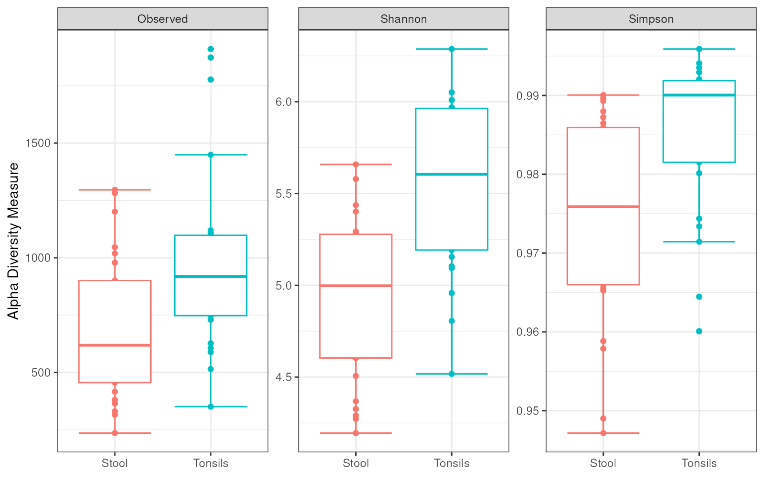
Beta Diversity Analysis

Beta diversity measures the taxonomic variation between samples by calculating the dissimilarity of clade relative abundances. The phyloseq package provides a method, distance, to calculate various dissimilarity measures, such as Bray–Curtis dissimilarity. Once dissimilarity has been calculated, samples can then be clustered and represented as a dendrogram.

V13_dendrogram <-
    distance(V13_phyloseq, method = "bray") %>%
    hclust() %>%
    as.dendrogram()

However, coercion to a dendrogram object results in the lost of sample_data present in the phyloseq object which is needed for plotting. A data.frame of this sample_data can be extracted from the phyloseq object as follows.

V13_sample_data <-
    sample_data(V13_phyloseq) %>%
    data.frame()

Samples in the the plots will be identified by “PSN”” (Primary Sample Number) and “Study”. So, additional columns to denote the colors and shapes of leaves and labels are added to the data.frame using dplyr syntax.

V13_sample_data %<>%
    rownames_to_column(var = "PSN") %>%
    mutate(labels_col = if_else(Study == "Stool", "#F8766D", "#00BFC4")) %>%
    mutate(leaves_col = if_else(Study == "Stool", "#F8766D", "#00BFC4")) %>%
    mutate(leaves_pch = if_else(Study == "Stool", 16, 17))

Additionally, the order of samples in the dendrogram and data.frame objects is different and a vector to sort samples is constructed as follows.

V13_sample_order <-
    labels(V13_dendrogram) %>%
    match(V13_sample_data$PSN)

The label and leaf color and shape columns of the data.frame object can then be coerced to vectors and sorted according to the sample order of the dendrogram object.

labels_col <- V13_sample_data$labels_col[V13_sample_order]
leaves_col <- V13_sample_data$leaves_col[V13_sample_order]
leaves_pch <- V13_sample_data$leaves_pch[V13_sample_order]

The dendextend package is then used to add these vectors to the dendrogram object as metadata which will be used for plotting.

V13_dendrogram %<>%
    set("labels_col", labels_col) %>%
    set("leaves_col", leaves_col) %>%
    set("leaves_pch", leaves_pch)

Finally, the dendextend package provides a method, circlize_dendrogram, to produce a circular dendrogram, using the circlize package, with a single line of code.

V13_dendrogram %>%
    circlize_dendrogram(labels_track_height = 0.2)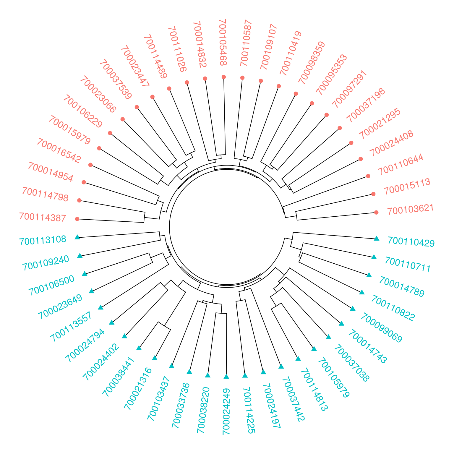

Principle Coordinates Analysis

The phyloseq package additionally provides methods for commonly-used ordination analyses such as principle coordinates analysis. The ordinate method simply requires a phyloseq object and specification of the type of ordination analysis to be preformed. The type of distance method used can also optionally be specified.

V13_ordination <-
    ordinate(V13_phyloseq, method = "PCoA", distance = "bray")

The ordination analysis can then be plotted using the plot_ordination method provided by the phyloseq package. Again, additional ggplot2 syntax is used to control the presentational aspects of the plot.

V13_phyloseq %>%
    plot_ordination(V13_ordination, color = "Study", shape = "Study") +
    theme_bw() +
    theme(legend.position = "bottom")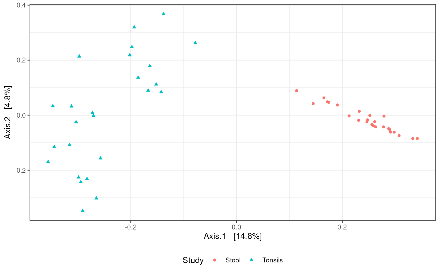

Finally, the ordination eigenvalues can be plotted using the plot_scree method provided by the phyloseq package.

V13_ordination %>%
    plot_scree() +
    theme_bw()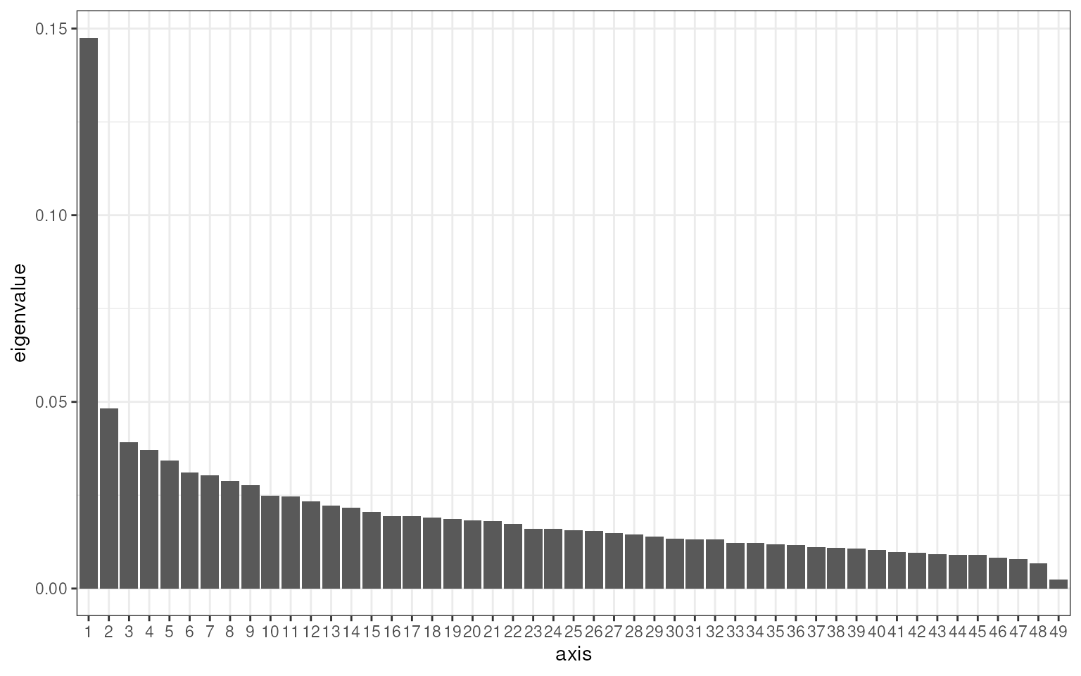

Phylum-level Comparison to Metagenomic Shotgun Sequencing

In addition to 16S rRNA sequencing, the HMP Study conducted whole metagenome shotgun (MGX) sequencing. These profiles, along with thousands of profiles from other studies, are available in the curatedMetagenomicData package. Here, a phylum-level relative abundance comparison of the 16S and MGX samples is made to illustrate comparing these data sets.

First a V35_stool_phyloseq object is constructed and contains the 16S variable region 3–5 data for stool samples. Then the MGX stool samples are obtained and coerced to a phyloseq object as follows.

V35_stool_phyloseq <-
    V35_stool %>%
    as_phyloseq()

EH <-
    ExperimentHub()

HMP_2012.metaphlan_bugs_list.stool <-
    EH[["EH426"]]

# a modified version of ExpressionSet2phyloseq taken from curatedMetagenomicData
# ExpressionSet2phyloseq was removed in curatedMetagenomicData version 3.0.0
ExpressionSet2phyloseq <- function(eset, simplify = TRUE, relab = TRUE) {
    otu.table <- 
        Biobase::exprs(eset)
    
    sample.data <-
        Biobase::pData(eset) %>%
        phyloseq::sample_data(., errorIfNULL = FALSE)

    taxonomic.ranks <-
        c("Kingdom", "Phylum", "Class", "Order", "Family", "Genus", "Species", "Strain")
    
    tax.table <-
        rownames(otu.table) %>%
        gsub("[a-z]__", "", .) %>%
        dplyr::tibble() %>%
        tidyr::separate(., ".", taxonomic.ranks, sep = "\\|", fill="right") %>%
        as.matrix()
    
    if(simplify) {
        rownames(otu.table) <- rownames(otu.table) %>%
            gsub(".+\\|", "", .)
    }
    
    rownames(tax.table) <-
        rownames(otu.table)
    
    if(!relab) {
        otu.table <-
            round(sweep(otu.table, 2, eset$number_reads/100, "*"))
    }
    
    otu.table <-
        phyloseq::otu_table(otu.table, taxa_are_rows = TRUE)
    
    tax.table <-
        phyloseq::tax_table(tax.table)
    
    
    phyloseq::phyloseq(otu.table, sample.data, tax.table)
}

MGX_stool_phyloseq <-
    ExpressionSet2phyloseq(HMP_2012.metaphlan_bugs_list.stool)

The curatedMetagenomicData package provides taxonomic relative abundance for MGX data (with an option to estimate counts by multiplying by read depth) from MetaPhlAn2. MetaPhlAn2 directly estimates relative abundance at every taxonomic level based on clade-specific markers, and these estimates are better than summing lower-level taxonomic abundances.

Note, this comparison becomes complicated because phyloseq does not currently support row and column matching and reordering. Instead, we use the phyloseq::psmelt() method to generate data.frame objects for further manipulation.

MGX_stool_melted <-
    MGX_stool_phyloseq %>%
    subset_taxa(is.na(Class) & !is.na(Phylum)) %>%
    psmelt()

The 16S data sets do not contain summarized counts for higher taxonomic levels, so we use the phyloseq::tax_glom() method to agglomerate at phylum level.

V35_stool_melted <-
    V35_stool_phyloseq %>%
    tax_glom(taxrank = "PHYLUM") %>%
    psmelt()

There is a column SRS_SAMPLE_ID present in the 16S variable region 3–5 data that is explicitly for mapping to the MGX samples and the matching identifiers are in the NCBI_accession column of the MGX sample data. The intersection of the two vectors represents the matching samples that are present in both data sets. This intersection, shown below as SRS_SAMPLE_IDS, can then be used to filter both the 16S and MGX samples to include only the samples in common.

Along with the filter step shown below, standardization of sample identifiers to the SRS numbers and conversion of taxonomic counts to relative abundance is done. The conversion to relative abundance is necessary for comparability across the 16S and MGX samples.

In either case, data is first grouped by samples and the percent composition of each phylum relative to the others in the sample is calculated by taking the count abundance of the phylum divided by the sum of all abundance counts in the sample. Samples are then sorted by phylum and descending relative abundance before being grouped by phylum – the grouping by phylum allows for the assignment a phylum rank that is then used to sort the phyla by descending relative abundance. Finally, only the sample, phylum, and relative abundance columns are kept once the order has been established and all groupings can be removed.

SRS_SAMPLE_IDS <-
    intersect(V35_stool_melted$SRS_SAMPLE_ID, MGX_stool_melted$NCBI_accession)

V35_stool_melted %<>%
    filter(SRS_SAMPLE_ID %in% SRS_SAMPLE_IDS) %>%
    rename(Phylum = PHYLUM) %>%
    mutate(Sample = SRS_SAMPLE_ID) %>%
    group_by(Sample) %>%
    mutate(`Relative Abundance` = Abundance / sum(Abundance)) %>%
    arrange(Phylum, -`Relative Abundance`) %>%
    group_by(Phylum) %>%
    mutate(phylum_rank = sum(`Relative Abundance`)) %>%
    arrange(-phylum_rank) %>%
    select(Sample, Phylum, `Relative Abundance`) %>%
    ungroup()

MGX_stool_melted %<>%
    filter(NCBI_accession %in% SRS_SAMPLE_IDS) %>%
    group_by(Sample) %>%
    mutate(`Relative Abundance` = Abundance / sum(Abundance)) %>%
    arrange(Phylum, -`Relative Abundance`) %>%
    group_by(Phylum) %>%
    mutate(phylum_rank = sum(`Relative Abundance`)) %>%
    arrange(-phylum_rank) %>%
    select(Sample, Phylum, `Relative Abundance`) %>%
    ungroup()

Provided that the phyla are ordered by relative abundance, the top phyla from each data set can be obtained and intersected to give the top eight phyla present in both data sets. The top eight phyla can then be used to filter 16S and MGX samples to include only the desired phyla.

V35_top_phyla <-
    V35_stool_melted %$%
    unique(Phylum) %>%
    as.character()

MGX_top_phyla <-
    MGX_stool_melted %$%
    unique(Phylum) %>%
    as.character()

top_eight_phyla <-
    intersect(V35_top_phyla, MGX_top_phyla) %>%
    extract(1:8)

V35_stool_melted %<>%
    filter(Phylum %in% top_eight_phyla)

MGX_stool_melted %<>%
    filter(Phylum %in% top_eight_phyla)

To achieve ordering of samples by the relative abundance of the top phylum when plotting, a vector of the unique sample identifiers is constructed and will be used as the levels of a factor.

sample_order <-
    V35_stool_melted %$%
    unique(Sample)

A vector of unique phyla is also constructed and will be used as the levels of a factor when plotting. If this were not done, phyla would simply be sorted alphabetically.

phylum_order <-
    V35_stool_melted %$%
    unique(Phylum)

Color blindness affects a significant portion of the population, but, using an intelligent color pallet, figures can be designed to be friendly to those with deuteranopia, protanopia, and tritanopia. The following colors are derived from Wong, B. Points of view: Color blindness. Nat. Methods 8, 441 (2011).

bang_wong_colors <-
    c("#CC79A7", "#D55E00", "#0072B2", "#F0E442", "#009E73", "#56B4E9",
      "#E69F00", "#000000")

Using the sample_order and phylum_order vectors constructed above, stacked phylum-level relative abundance bar plots sorted by decreasing relative abundance of the top phylum and stratified by the top eight phyla can be made for 16S and MGX samples. The two plots are made separately and serialized so that they can be arranged in a single figure for comparison.

V35_plot <-
    V35_stool_melted %>%
    mutate(Sample = factor(Sample, sample_order)) %>%
    mutate(Phylum = factor(Phylum, phylum_order)) %>%
    ggplot(aes(Sample, `Relative Abundance`, fill = Phylum)) +
    geom_bar(stat = "identity", position = "fill", width = 1) +
    scale_fill_manual(values = bang_wong_colors) +
    theme_minimal() +
    theme(axis.text.x = element_blank(), axis.title.x = element_blank(),
          panel.grid = element_blank(), legend.position = "none",
          legend.title = element_blank()) +
    ggtitle("Phylum-Level Relative Abundance", "16S Stool Samples")

MGX_plot <-
    MGX_stool_melted %>%
    mutate(Sample = factor(Sample, sample_order)) %>%
    mutate(Phylum = factor(Phylum, phylum_order)) %>%
    ggplot(aes(Sample, `Relative Abundance`, fill = Phylum)) +
    geom_bar(stat = "identity", position = "fill", width = 1) +
    scale_fill_manual(values = bang_wong_colors) +
    theme_minimal() +
    theme(axis.text.x = element_blank(), axis.title.x = element_blank(),
          panel.grid = element_blank(), legend.position = "none",
          legend.title = element_blank()) +
    ggtitle("", "MGX Stool Samples")

In the plots above, legends are removed to reduce redundancy, but a legend is still necessary and can be serialized as its own plot using the get_legend method from the cowplot package.

plot_legend <- {
        MGX_plot +
            theme(legend.position = "bottom")
    } %>%
    get_legend()

## Warning in get_plot_component(plot, "guide-box"): Multiple components found;
## returning the first one. To return all, use `return_all = TRUE`.

Finally, the grid.arrange method from the gridExtra package is used to arrange, scale, and plot the three plots in a single figure.

grid.arrange(V35_plot, MGX_plot, plot_legend, ncol = 1, heights = c(3, 3, 1))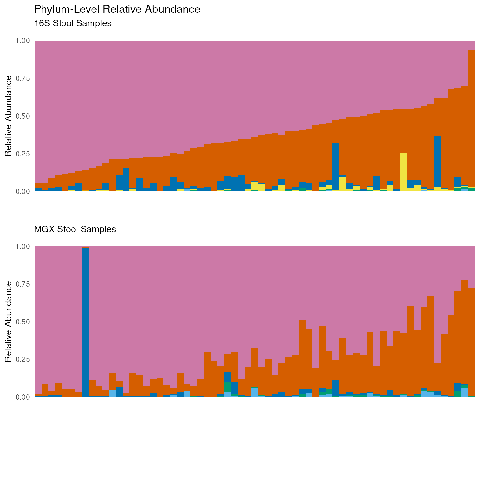

Notably, the figure illustrates the Bacteroidetes/Firmicutes gradient with reasonable agreement between the 16S and MGX samples.

When these plots were submitted for publication, the following code was used to produce ESP and PDF files.

V35_plot +
    theme(text = element_text(size = 19)) +
    labs(title = NULL, subtitle = NULL, tag = "A")

ggsave("~/AJE-00611-2018 Schiffer Figure 2A.eps", device = "eps")
ggsave("~/AJE-00611-2018 Schiffer Figure 2A.pdf", device = "pdf")

MGX_plot +
    theme(text = element_text(size = 19)) +
    labs(title = NULL, subtitle = NULL, tag = "B")

ggsave("~/AJE-00611-2018 Schiffer Figure 2B.eps", device = "eps")
ggsave("~/AJE-00611-2018 Schiffer Figure 2B.pdf", device = "pdf")

plot_legend <- {
        MGX_plot +
            theme(legend.position = "bottom", text = element_text(size = 19)) +
            guides(fill = guide_legend(byrow = TRUE))
    } %>%
    get_legend()

ggsave("~/AJE-00611-2018 Schiffer Figure 2 Legend 1.eps", plot = plot_legend,
       device = "eps")
ggsave("~/AJE-00611-2018 Schiffer Figure 2 Legend 1.pdf", plot = plot_legend,
       device = "pdf")

plot_legend <- {
        MGX_plot +
            theme(legend.position = "right", text = element_text(size = 19))
    } %>%
    get_legend()

ggsave("~/AJE-00611-2018 Schiffer Figure 2 Legend 2.eps", plot = plot_legend,
       device = "eps")
ggsave("~/AJE-00611-2018 Schiffer Figure 2 Legend 2.pdf", plot = plot_legend,
       device = "pdf")

plot_legend <- {
        MGX_plot +
            theme(legend.position = "right", text = element_text(size = 19)) +
            guides(fill = guide_legend(ncol = 2, byrow = TRUE))
    } %>%
    get_legend()

ggsave("~/AJE-00611-2018 Schiffer Figure 2 Legend 3.eps", plot = plot_legend,
       device = "eps")
ggsave("~/AJE-00611-2018 Schiffer Figure 2 Legend 3.pdf", plot = plot_legend,
       device = "pdf")

V35_plot <-
    V35_plot +
    theme(text = element_text(size = 19)) +
    labs(title = NULL, subtitle = NULL, tag = "A")

MGX_plot <-
    MGX_plot +
    theme(text = element_text(size = 19)) +
    labs(title = NULL, subtitle = NULL, tag = "B")

plot_legend <- {
        MGX_plot +
            theme(legend.position = "bottom", text = element_text(size = 19)) +
            guides(fill = guide_legend(byrow = TRUE))
    } %>%
    get_legend()

grid_object <-
    grid.arrange(V35_plot, MGX_plot, plot_legend, ncol = 1,
                 heights = c(3, 3, 1))

ggsave("~/AJE-00611-2018 Schiffer Figure 3.eps", plot = grid_object,
       device = "eps", width = 8, height = 8)
ggsave("~/AJE-00611-2018 Schiffer Figure 3.pdf", plot = grid_object,
       device = "pdf", width = 8, height = 8)

Exporting Data to CSV, SAS, SPSS, and STATA Formats

To our knowledge, R and Bioconductor provide the most and best methods for the analysis of microbiome data. However, we realize they are not the only analysis environments and wish to provide methods to export the data from HMP16SData to CSV, SAS, SPSS, and STATA formats. As we do not use these other languages regularly, we are unaware of how to represent phylogenitic trees in them and will not attempt to export the trees here.

Prepare Data for Export

Bioconductor’s SummarizedExperiment class is essentially a normalized representation of tightly coupled data and metadata that must be “unglued” before it can be saved into alternative formats.

The process begins by creating a data.frame object of the participant data and moving the row names to their own column.

V13_participant_data <-
  V13() %>%
  colData() %>%
  as.data.frame() %>%
  rownames_to_column(var = "PSN")

Next, the taxonomic abundance matrix is extracted and transposed because Bioconductor objects represent samples as rows and measurements as columns whereas other languages do the opposite. The matrix is then coerced to a data.frame object and the row names are moved to their own column.

V13_OTU_counts <-
  V13() %>%
  assay() %>%
  t() %>%
  as.data.frame() %>%
  rownames_to_column(var = "PSN")

With the participant data and taxonomic abundances represented as simple tables containing a primary key (i.e. PSN or Primary Sample Number) the two tables can be joined using the merge.data.frame method.

V13_data <-
  merge.data.frame(V13_participant_data, V13_OTU_counts, by = "PSN")

The column names of the V13_data object are denoted as OTUs or operational taxonomic units based on their sequence similarity to the 16S rRNA gene. The OTU nomenclature is not particularly useful without the traditional taxonomic clade identifiers which are stored in a separate table. A dictionary of these identifiers is created by extracting and transposing the rowData of the SummarizedExperiment object which is then coerced to a data.frame object.

V13_dictionary <-
  V13() %>%
  rowData() %>%
  t.data.frame() %>%
  as.data.frame()

The column names of the V13_data object contain periods which some languages and formats are unable to process. The periods in the column names are replaced with underscores using the gsub method.

colnames(V13_data) <-
    colnames(V13_data) %>%
    gsub(pattern = "\\.", replacement = "_", x = .)

The process is repeated for the column names of the V13_dictionary object.

colnames(V13_dictionary) <-
    colnames(V13_dictionary) %>%
    gsub(pattern = "\\.", replacement = "_", x = .)

The two tables V13_data and V13_dictionary are then ready for export to CSV, SAS, SPSS, and STATA formats.

Export to CSV Format

To export to CSV format, two calls to the write_csv method from the readr package are used to write CSV files to disk.

write_csv(V13_data, "~/V13_data.csv")
write_csv(V13_dictionary, "~/V13_dictionary.csv")

Export to SAS Format

To export to SAS format, two calls to the write_sas method from the haven package are used to write SAS files to disk.

write_sas(V13_data, "~/V13_data.sas7bdat")
write_sas(V13_dictionary, "~/V13_dictionary.sas7bdat")

Export to SPSS Format

To export to SPSS format, two calls to the write_sav method from the haven package are used to write SPSS files to disk.

write_sav(V13_data, "~/V13_data.sav")
write_sav(V13_dictionary, "~/V13_dictionary.sav")

Export to STATA Format

To export to STATA format, two calls to the write_dta method from the haven package are used to write STATA files to disk.

write_dta(V13_data, "~/V13_data.dta", version = 13)
write_dta(V13_dictionary, "~/V13_dictionary.dta", version = 13)

Here, version 13 STATA files are written because version 14 and above files require a platform-specific text encoding that would make the data less transportable. The encoding of the version 13 files is ASCII.

Session Information

sessionInfo()

## R version 4.5.0 (2025-04-11)
## Platform: x86_64-pc-linux-gnu
## Running under: Ubuntu 24.04.2 LTS
## 
## Matrix products: default
## BLAS:   /usr/lib/x86_64-linux-gnu/openblas-pthread/libblas.so.3 
## LAPACK: /usr/lib/x86_64-linux-gnu/openblas-pthread/libopenblasp-r0.3.26.so;  LAPACK version 3.12.0
## 
## locale:
##  [1] LC_CTYPE=en_US.UTF-8       LC_NUMERIC=C              
##  [3] LC_TIME=en_US.UTF-8        LC_COLLATE=en_US.UTF-8    
##  [5] LC_MONETARY=en_US.UTF-8    LC_MESSAGES=en_US.UTF-8   
##  [7] LC_PAPER=en_US.UTF-8       LC_NAME=C                 
##  [9] LC_ADDRESS=C               LC_TELEPHONE=C            
## [11] LC_MEASUREMENT=en_US.UTF-8 LC_IDENTIFICATION=C       
## 
## time zone: Etc/UTC
## tzcode source: system (glibc)
## 
## attached base packages:
## [1] stats4    stats     graphics  grDevices utils     datasets  methods  
## [8] base     
## 
## other attached packages:
##  [1] haven_2.5.4                 readr_2.1.5                
##  [3] cowplot_1.1.3               gridExtra_2.3              
##  [5] ExperimentHub_2.16.0        AnnotationHub_3.16.0       
##  [7] BiocFileCache_2.16.0        dbplyr_2.5.0               
##  [9] circlize_0.4.16             dendextend_1.19.0          
## [11] dplyr_1.1.4                 tibble_3.2.1               
## [13] ggplot2_3.5.2               magrittr_2.0.3             
## [15] phyloseq_1.52.0             HMP16SData_1.28.0          
## [17] SummarizedExperiment_1.38.1 Biobase_2.68.0             
## [19] GenomicRanges_1.60.0        GenomeInfoDb_1.44.0        
## [21] IRanges_2.42.0              S4Vectors_0.46.0           
## [23] BiocGenerics_0.54.0         generics_0.1.3             
## [25] MatrixGenerics_1.20.0       matrixStats_1.5.0          
## [27] BiocStyle_2.36.0           
## 
## loaded via a namespace (and not attached):
##   [1] RColorBrewer_1.1-3      rstudioapi_0.17.1       jsonlite_2.0.0         
##   [4] shape_1.4.6.1           farver_2.1.2            rmarkdown_2.29         
##   [7] GlobalOptions_0.1.2     fs_1.6.6                ragg_1.4.0             
##  [10] vctrs_0.6.5             multtest_2.64.0         memoise_2.0.1          
##  [13] htmltools_0.5.8.1       S4Arrays_1.8.0          forcats_1.0.0          
##  [16] curl_6.2.2              Rhdf5lib_1.30.0         SparseArray_1.8.0      
##  [19] rhdf5_2.52.0            sass_0.4.10             bslib_0.9.0            
##  [22] htmlwidgets_1.6.4       desc_1.4.3              plyr_1.8.9             
##  [25] cachem_1.1.0            igraph_2.1.4            mime_0.13              
##  [28] lifecycle_1.0.4         iterators_1.0.14        pkgconfig_2.0.3        
##  [31] Matrix_1.7-3            R6_2.6.1                fastmap_1.2.0          
##  [34] GenomeInfoDbData_1.2.14 digest_0.6.37           colorspace_2.1-1       
##  [37] AnnotationDbi_1.70.0    textshaping_1.0.1       RSQLite_2.3.11         
##  [40] vegan_2.6-10            labeling_0.4.3          filelock_1.0.3         
##  [43] httr_1.4.7              abind_1.4-8             mgcv_1.9-3             
##  [46] compiler_4.5.0          bit64_4.6.0-1           withr_3.0.2            
##  [49] viridis_0.6.5           DBI_1.2.3               MASS_7.3-65            
##  [52] rappdirs_0.3.3          DelayedArray_0.34.1     biomformat_1.36.0      
##  [55] permute_0.9-7           tools_4.5.0             ape_5.8-1              
##  [58] glue_1.8.0              nlme_3.1-168            rhdf5filters_1.20.0    
##  [61] grid_4.5.0              cluster_2.1.8.1         reshape2_1.4.4         
##  [64] ade4_1.7-23             gtable_0.3.6            tzdb_0.5.0             
##  [67] tidyr_1.3.1             data.table_1.17.0       hms_1.1.3              
##  [70] xml2_1.3.8              XVector_0.48.0          BiocVersion_3.21.1     
##  [73] foreach_1.5.2           pillar_1.10.2           stringr_1.5.1          
##  [76] splines_4.5.0           lattice_0.22-7          survival_3.8-3         
##  [79] bit_4.6.0               tidyselect_1.2.1        Biostrings_2.76.0      
##  [82] knitr_1.50              bookdown_0.43           svglite_2.1.3          
##  [85] xfun_0.52               stringi_1.8.7           UCSC.utils_1.4.0       
##  [88] yaml_2.3.10             kableExtra_1.4.0        evaluate_1.0.3         
##  [91] codetools_0.2-20        BiocManager_1.30.25     cli_3.6.5              
##  [94] systemfonts_1.2.3       jquerylib_0.1.4         Rcpp_1.0.14            
##  [97] png_0.1-8               parallel_4.5.0          pkgdown_2.1.2          
## [100] assertthat_0.2.1        blob_1.2.4              viridisLite_0.4.2      
## [103] scales_1.4.0            purrr_1.0.4             crayon_1.5.3           
## [106] rlang_1.1.6             KEGGREST_1.48.0