Installation

If you are using the Docker container provided with this workshop, everything (including the workshop) is already installed. Otherwise, you will need to install the following packages.

required_pkgs = c(
  "GEOquery", 
  "GenomicDataCommons",
  "curatedTCGAData",
  "TCGAutils",
  "cBioPortalData",
  "recount",
  "curatedMetagenomicData",
  "phyloseq",
  "HMP16SData",
  "PharmacoGx")
BiocManager::install(required_pkgs)

Sean Davis

GEOquery

(Davis and Meltzer 2007)

The NCBI Gene Expression Omnibus (GEO) serves as a public repository for a wide range of high-throughput experimental data. These data include single and dual channel microarray-based experiments measuring mRNA, genomic DNA, and protein abundance, as well as non-array techniques such as serial analysis of gene expression (SAGE), mass spectrometry proteomic data, and high-throughput sequencing data. The GEOquery package (Davis and Meltzer 2007) forms a bridge between this public repository and the analysis capabilities in Bioconductor.

Overview of GEO

At the most basic level of organization of GEO, there are four basic entity types. The first three (Sample, Platform, and Series) are supplied by users; the fourth, the dataset, is compiled and curated by GEO staff from the user-submitted data. See the GEO home page for more information.

Platforms

A Platform record describes the list of elements on the array (e.g., cDNAs, oligonucleotide probesets, ORFs, antibodies) or the list of elements that may be detected and quantified in that experiment (e.g., SAGE tags, peptides). Each Platform record is assigned a unique and stable GEO accession number (GPLxxx). A Platform may reference many Samples that have been submitted by multiple submitters.

Samples

A Sample record describes the conditions under which an individual Sample was handled, the manipulations it underwent, and the abundance measurement of each element derived from it. Each Sample record is assigned a unique and stable GEO accession number (GSMxxx). A Sample entity must reference only one Platform and may be included in multiple Series.

Series

A Series record defines a set of related Samples considered to be part of a group, how the Samples are related, and if and how they are ordered. A Series provides a focal point and description of the experiment as a whole. Series records may also contain tables describing extracted data, summary conclusions, or analyses. Each Series record is assigned a unique and stable GEO accession number (GSExxx). Series records are available in a couple of formats which are handled by GEOquery independently. The smaller and new GSEMatrix files are quite fast to parse; a simple flag is used by GEOquery to choose to use GSEMatrix files (see below).

Datasets

GEO DataSets (GDSxxx) are curated sets of GEO Sample data. There are hundreds of GEO datasets available, but GEO discontinued creating GDS records several years ago. We mention them here for completeness only.

Getting Started using GEOquery

Getting data from GEO is really quite easy. There is only one command that is needed, getGEO. This one function interprets its input to determine how to get the data from GEO and then parse the data into useful R data structures.

library(GEOquery)

With the library loaded, we are free to access any GEO accession.

Use case: MDS plot of cancer data

The data we are going to access are from this paper.

Background: The tumor microenvironment is an important factor in cancer immunotherapy response. To further understand how a tumor affects the local immune system, we analyzed immune gene expression differences between matching normal and tumor tissue.Methods: We analyzed public and new gene expression data from solid cancers and isolated immune cell populations. We also determined the correlation between CD8, FoxP3 IHC, and our gene signatures.Results: We observed that regulatory T cells (Tregs) were one of the main drivers of immune gene expression differences between normal and tumor tissue. A tumor-specific CD8 signature was slightly lower in tumor tissue compared with normal of most (12 of 16) cancers, whereas a Treg signature was higher in tumor tissue of all cancers except liver. Clustering by Treg signature found two groups in colorectal cancer datasets. The high Treg cluster had more samples that were consensus molecular subtype 1/4, right-sided, and microsatellite-instable, compared with the low Treg cluster. Finally, we found that the correlation between signature and IHC was low in our small dataset, but samples in the high Treg cluster had significantly more CD8+ and FoxP3+ cells compared with the low Treg cluster.Conclusions: Treg gene expression is highly indicative of the overall tumor immune environment.Impact: In comparison with the consensus molecular subtype and microsatellite status, the Treg signature identifies more colorectal tumors with high immune activation that may benefit from cancer immunotherapy.

In this little exercise, we will:

1. Access public omics data using the GEOquery package
2. Convert the public omics data to a SummarizedExperiment object.
3. Perform a simple unsupervised analysis to visualize these public data.

Use the GEOquery package to fetch data about GSE103512.

gse = getGEO("GSE103512")[[1]]

## Warning: 102 parsing failures.
##   row     col           expected    actual         file
## 54614 SPOT_ID 1/0/T/F/TRUE/FALSE --Control literal data
## 54615 SPOT_ID 1/0/T/F/TRUE/FALSE --Control literal data
## 54616 SPOT_ID 1/0/T/F/TRUE/FALSE --Control literal data
## 54617 SPOT_ID 1/0/T/F/TRUE/FALSE --Control literal data
## 54618 SPOT_ID 1/0/T/F/TRUE/FALSE --Control literal data
## ..... ....... .................. ......... ............
## See problems(...) for more details.

Note that getGEO, when used to retrieve GSE records, returns a list. The members of the list each represent one GEO Platform, since each GSE record can contain multiple related datasets (eg., gene expression and DNA methylation). In this case, the list is of length one, but it is still necessary to grab the first elment.

The first step–a detail–is to convert from the older Bioconductor data structure (GEOquery was written in 2007), the ExpressionSet, to the newer SummarizedExperiment. One line suffices.

library(SummarizedExperiment)
se = as(gse, "SummarizedExperiment")

Examine two variables of interest, cancer type and tumor/normal status.

with(colData(se),table(`cancer.type.ch1`,`normal.ch1`))

##                normal.ch1
## cancer.type.ch1 no yes
##           BC    65  10
##           CRC   57  12
##           NSCLC 60   9
##           PCA   60   7

Filter gene expression by variance to find most informative genes.

sds = apply(assay(se, 'exprs'),1,sd)
dat = assay(se, 'exprs')[order(sds,decreasing = TRUE)[1:500],]

Perform multidimensional scaling and prepare for plotting. We will be using ggplot2, so we need to make a data.frame before plotting.

mdsvals = cmdscale(dist(t(dat)))
mdsvals = as.data.frame(mdsvals)
mdsvals$Type=factor(colData(se)[,'cancer.type.ch1'])
mdsvals$Normal = factor(colData(se)[,'normal.ch1'])
head(mdsvals)

##                   V1       V2 Type Normal
## GSM2772660  8.531331 18.57115   BC     no
## GSM2772661  8.991591 13.63764   BC     no
## GSM2772662 10.788973 13.48403   BC     no
## GSM2772663  3.127105 19.13529   BC     no
## GSM2772664 13.056599 13.88711   BC     no
## GSM2772665  7.903717 13.24731   BC     no

And do the plot.

library(ggplot2)
ggplot(mdsvals, aes(x=V1,y=V2,shape=Normal,color=Type)) + 
    geom_point( alpha=0.6) + theme(text=element_text(size = 18))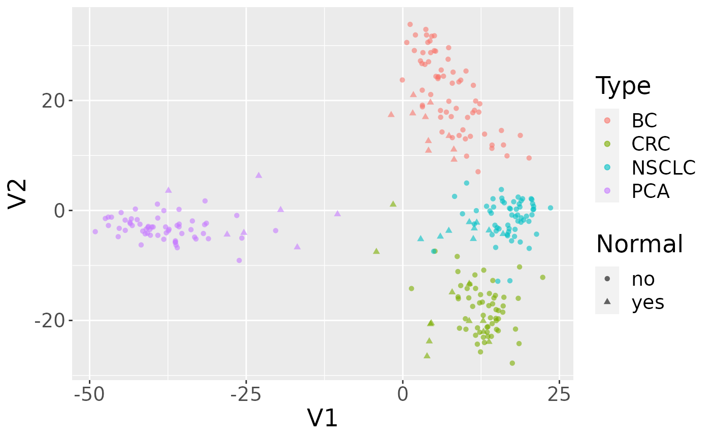

Accessing Raw Data from GEO

NCBI GEO accepts (but has not always required) raw data such as .CEL files, .CDF files, images, etc. It is also not uncommon for some RNA-seq or other sequencing datasets to supply only raw data (with accompanying sample information, of course), necessitating Sometimes, it is useful to get quick access to such data. A single function, getGEOSuppFiles, can take as an argument a GEO accession and will download all the raw data associate with that accession. By default, the function will create a directory in the current working directory to store the raw data for the chosen GEO accession.

GenomicDataCommons

From the Genomic Data Commons (GDC) website:

The National Cancer Institute’s (NCI’s) Genomic Data Commons (GDC) is a data sharing platform that promotes precision medicine in oncology. It is not just a database or a tool; it is an expandable knowledge network supporting the import and standardization of genomic and clinical data from cancer research programs. The GDC contains NCI-generated data from some of the largest and most comprehensive cancer genomic datasets, including The Cancer Genome Atlas (TCGA) and Therapeutically Applicable Research to Generate Effective Therapies (TARGET). For the first time, these datasets have been harmonized using a common set of bioinformatics pipelines, so that the data can be directly compared. As a growing knowledge system for cancer, the GDC also enables researchers to submit data, and harmonizes these data for import into the GDC. As more researchers add clinical and genomic data to the GDC, it will become an even more powerful tool for making discoveries about the molecular basis of cancer that may lead to better care for patients.

The data model for the GDC is complex, but it worth a quick overview and a graphical representation is included here.

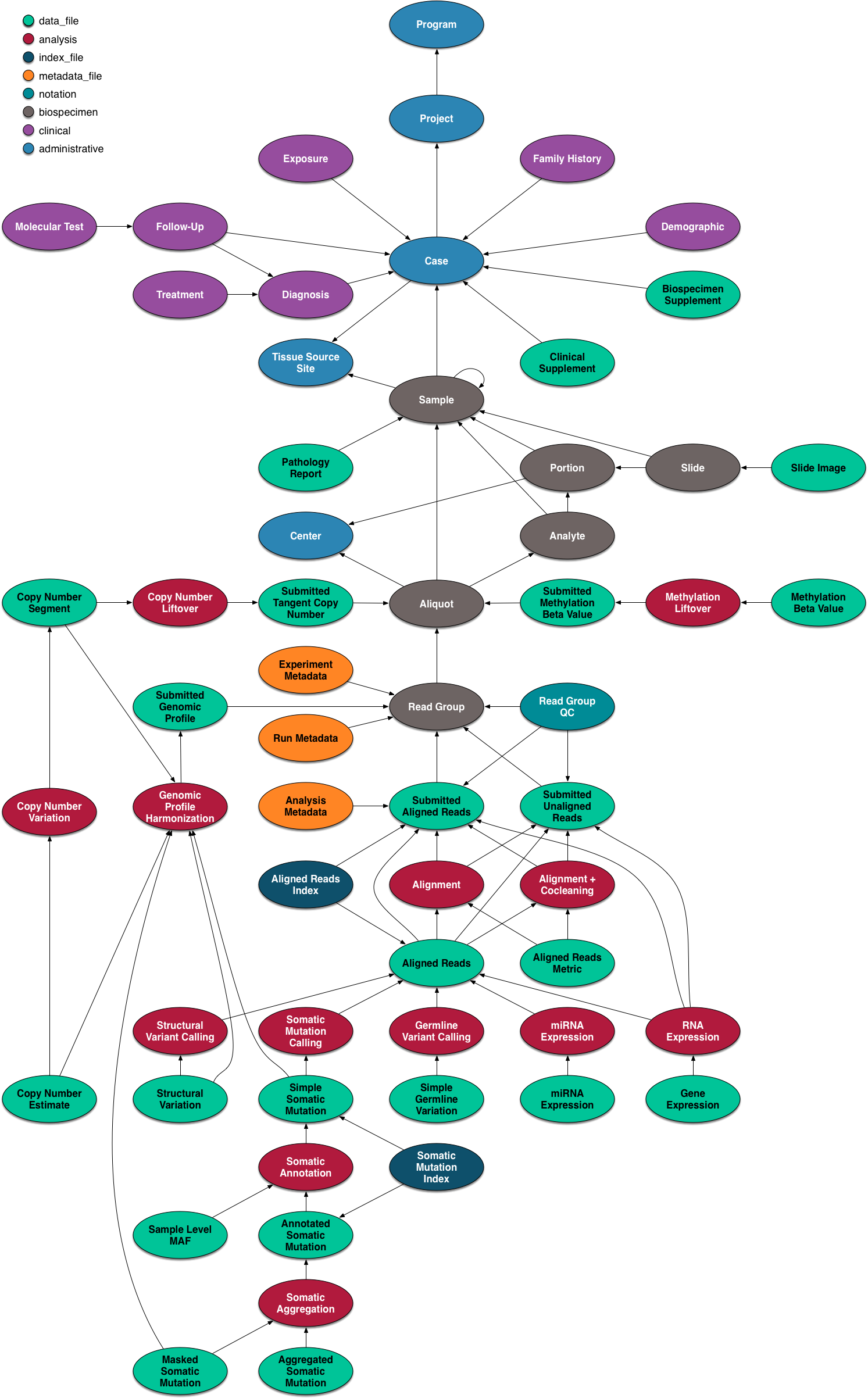
The data model is encoded as a so-called property graph. Nodes represent entities such as Projects, Cases, Diagnoses, Files (various kinds), and Annotations. The relationships between these entities are maintained as edges. Both nodes and edges may have Properties that supply instance details.

The GDC API exposes these nodes and edges in a somewhat simplified set of RESTful endpoints.

Quickstart

This quickstart section is just meant to show basic functionality. More details of functionality are included further on in this vignette and in function-specific help.

To report bugs or problems, either submit a new issue or submit a bug.report(package='GenomicDataCommons') from within R (which will redirect you to the new issue on GitHub).

library(GenomicDataCommons)

Check connectivity and status

The GenomicDataCommons package relies on having network connectivity. In addition, the NCI GDC API must also be operational and not under maintenance. Checking status can be used to check this connectivity and functionality.

GenomicDataCommons::status()

## $commit
## [1] "dfa394478bd39c11b89d3819a398898d99575a24"
## 
## $data_release
## [1] "Data Release 29.0 - March 31, 2021"
## 
## $status
## [1] "OK"
## 
## $tag
## [1] "3.0.0"
## 
## $version
## [1] 1

Find data

The following code builds a manifest that can be used to guide the download of raw data. Here, filtering finds gene expression files quantified as raw counts using HTSeq from ovarian cancer patients.

library(magrittr)
ge_manifest = files() %>%
    filter( ~ cases.project.project_id == 'TCGA-OV' &
                type == 'gene_expression' &
                analysis.workflow_type == 'HTSeq - Counts') %>%
    manifest()

Download data

After the 379 gene expression files specified in the query above. Using multiple processes to do the download very significantly speeds up the transfer in many cases. On a standard 1Gb connection, the following completes in about 30 seconds. The first time the data are downloaded, R will ask to create a cache directory (see ?gdc_cache for details of setting and interacting with the cache). Resulting downloaded files will be stored in the cache directory. Future access to the same files will be directly from the cache, alleviating multiple downloads.

fnames = lapply(ge_manifest$id[1:20],gdcdata)

If the download had included controlled-access data, the download above would have needed to include a token. Details are available in the authentication section below.

Metadata queries

The GenomicDataCommons can access the significant clinical, demographic, biospecimen, and annotation information contained in the NCI GDC.

expands = c("diagnoses","annotations",
             "demographic","exposures")
projResults = projects() %>%
    results(size=10)
str(projResults,list.len=5)

## List of 9
##  $ id                    : chr [1:10] "GENIE-MSK" "TCGA-UCEC" "TCGA-LGG" "TCGA-SARC" ...
##  $ primary_site          :List of 10
##   ..$ GENIE-MSK : chr [1:49] "Testis" "Gallbladder" "Unknown" "Other and unspecified parts of biliary tract" ...
##   ..$ TCGA-UCEC : chr [1:2] "Corpus uteri" "Uterus, NOS"
##   ..$ TCGA-LGG  : chr "Brain"
##   ..$ TCGA-SARC : chr [1:13] "Kidney" "Other and unspecified parts of tongue" "Bones, joints and articular cartilage of limbs" "Colon" ...
##   ..$ TCGA-PAAD : chr "Pancreas"
##   .. [list output truncated]
##  $ dbgap_accession_number: logi [1:10] NA NA NA NA NA NA ...
##  $ project_id            : chr [1:10] "GENIE-MSK" "TCGA-UCEC" "TCGA-LGG" "TCGA-SARC" ...
##  $ disease_type          :List of 10
##   ..$ GENIE-MSK : chr [1:49] "Germ Cell Neoplasms" "Granular Cell Tumors and Alveolar Soft Part Sarcomas" "Immunoproliferative Diseases" "Plasma Cell Tumors" ...
##   ..$ TCGA-UCEC : chr [1:4] "Epithelial Neoplasms, NOS" "Cystic, Mucinous and Serous Neoplasms" "Adenomas and Adenocarcinomas" "Not Reported"
##   ..$ TCGA-LGG  : chr "Gliomas"
##   ..$ TCGA-SARC : chr [1:6] "Nerve Sheath Tumors" "Myomatous Neoplasms" "Fibromatous Neoplasms" "Lipomatous Neoplasms" ...
##   ..$ TCGA-PAAD : chr [1:4] "Cystic, Mucinous and Serous Neoplasms" "Ductal and Lobular Neoplasms" "Adenomas and Adenocarcinomas" "Epithelial Neoplasms, NOS"
##   .. [list output truncated]
##   [list output truncated]
##  - attr(*, "row.names")= int [1:10] 1 2 3 4 5 6 7 8 9 10
##  - attr(*, "class")= chr [1:3] "GDCprojectsResults" "GDCResults" "list"

names(projResults)

## [1] "id"                     "primary_site"           "dbgap_accession_number"
## [4] "project_id"             "disease_type"           "name"                  
## [7] "releasable"             "state"                  "released"

# or listviewer::jsonedit(clinResults)

Basic design

This package design is meant to have some similarities to the “hadleyverse” approach of dplyr. Roughly, the functionality for finding and accessing files and metadata can be divided into:

1. Simple query constructors based on GDC API endpoints.
2. A set of verbs that when applied, adjust filtering, field selection, and faceting (fields for aggregation) and result in a new query object (an endomorphism)
3. A set of verbs that take a query and return results from the GDC

In addition, there are exhiliary functions for asking the GDC API for information about available and default fields, slicing BAM files, and downloading actual data files. Here is an overview of functionality¹.

• Creating a query
  • projects()
  • cases()
  • files()
  • annotations()
• Manipulating a query
  • filter()
  • facet()
  • select()
• Introspection on the GDC API fields
  • mapping()
  • available_fields()
  • default_fields()
  • grep_fields()
  • field_picker()
  • available_values()
  • available_expand()
• Executing an API call to retrieve query results
  • results()
  • count()
  • response()
• Raw data file downloads
  • gdcdata()
  • transfer()
  • gdc_client()
• Summarizing and aggregating field values (faceting)
  • aggregations()
• Authentication
  • gdc_token()
• BAM file slicing
  • slicing()

Usage

There are two main classes of operations when working with the NCI GDC.

1. Querying metadata and finding data files (e.g., finding all gene expression quantifications data files for all colon cancer patients).
2. Transferring raw or processed data from the GDC to another computer (e.g., downloading raw or processed data)

Both classes of operation are reviewed in detail in the following sections.

Querying metadata

Vast amounts of metadata about cases (patients, basically), files, projects, and so-called annotations are available via the NCI GDC API. Typically, one will want to query metadata to either focus in on a set of files for download or transfer or to perform so-called aggregations (pivot-tables, facets, similar to the R table() functionality).

Querying metadata starts with creating a “blank” query. One will often then want to filter the query to limit results prior to retrieving results. The GenomicDataCommons package has helper functions for listing fields that are available for filtering.

In addition to fetching results, the GDC API allows faceting, or aggregating,, useful for compiling reports, generating dashboards, or building user interfaces to GDC data (see GDC web query interface for a non-R-based example).

Creating a query

The GenomicDataCommons package accesses the same API as the GDC website. Therefore, a useful approach, particularly for beginning users is to examine the filters available on the GDC repository pages to find appropriate filtering criteria. From there, converting those checkboxes to a GenomicDataCommons query() is relatively straightforward. Note that only a small subset of the available_fields() are available by default on the website.

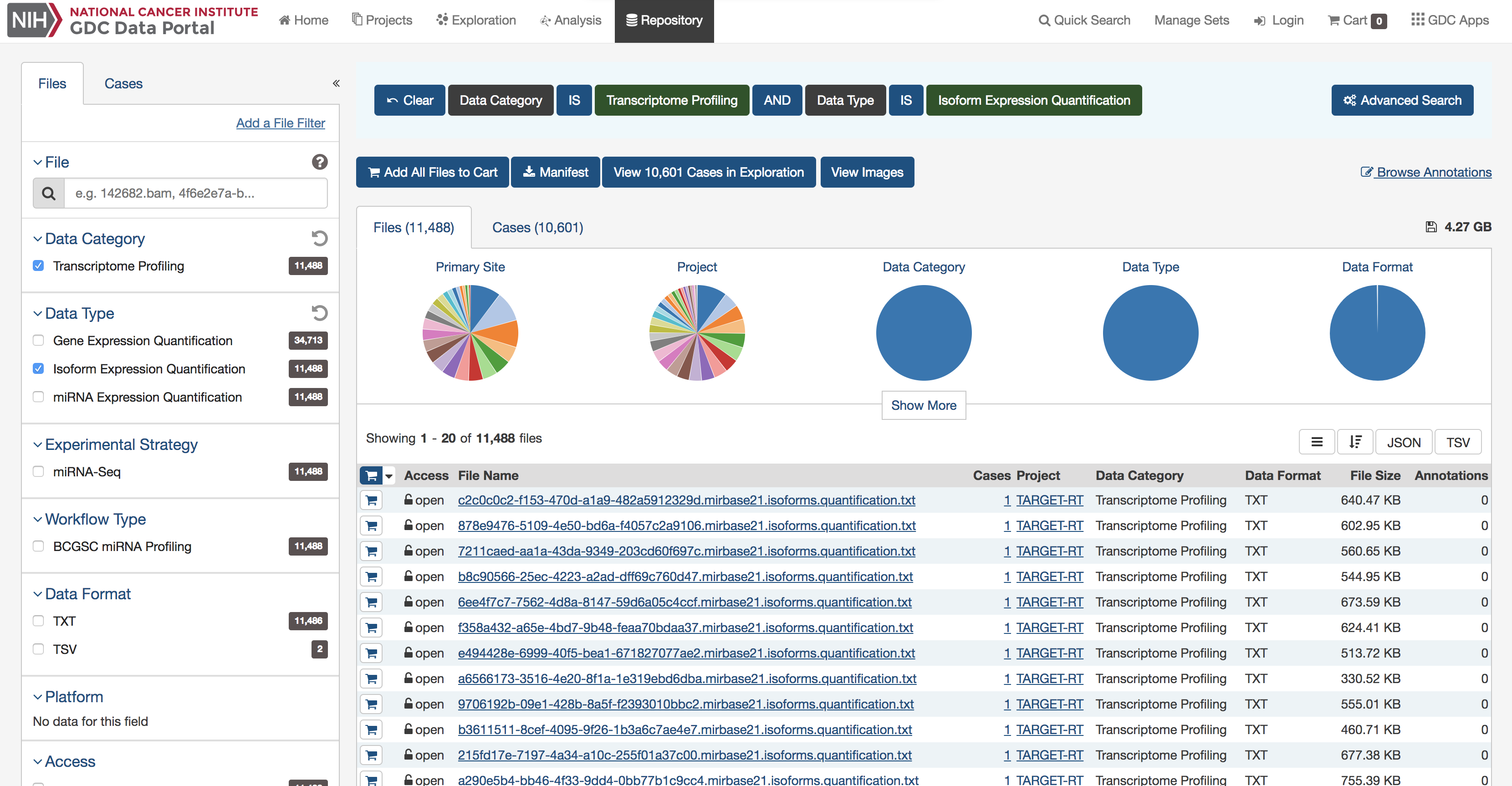
A screenshot of an example query of the GDC repository portal.

A query of the GDC starts its life in R. Queries follow the four metadata endpoints available at the GDC. In particular, there are four convenience functions that each create GDCQuery objects (actually, specific subclasses of GDCQuery):

• projects()
• cases()
• files()
• annotations()

pquery = projects()

The pquery object is now an object of (S3) class, GDCQuery (and gdc_projects and list). The object contains the following elements:

• fields: This is a character vector of the fields that will be returned when we retrieve data. If no fields are specified to, for example, the projects() function, the default fields from the GDC are used (see default_fields())
• filters: This will contain results after calling the filter() method and will be used to filter results on retrieval.
• facets: A character vector of field names that will be used for aggregating data in a call to aggregations().
• archive: One of either “default” or “legacy”.
• token: A character(1) token from the GDC. See the authentication section for details, but note that, in general, the token is not necessary for metadata query and retrieval, only for actual data download.

Looking at the actual object (get used to using str()!), note that the query contains no results.

str(pquery)

## List of 5
##  $ fields : chr [1:10] "dbgap_accession_number" "disease_type" "intended_release_date" "name" ...
##  $ filters: NULL
##  $ facets : NULL
##  $ legacy : logi FALSE
##  $ expand : NULL
##  - attr(*, "class")= chr [1:3] "gdc_projects" "GDCQuery" "list"

Retrieving results

[ GDC pagination documentation ]

[ GDC sorting documentation ]

With a query object available, the next step is to retrieve results from the GDC. The GenomicDataCommons package. The most basic type of results we can get is a simple count() of records available that satisfy the filter criteria. Note that we have not set any filters, so a count() here will represent all the project records publicly available at the GDC in the “default” archive"

pcount = count(pquery)
# or
pcount = pquery %>% count()
pcount

## [1] 68

The results() method will fetch actual results.

presults = pquery %>% results()

These results are returned from the GDC in JSON format and converted into a (potentially nested) list in R. The str() method is useful for taking a quick glimpse of the data.

str(presults)

## List of 9
##  $ id                    : chr [1:10] "GENIE-MSK" "TCGA-UCEC" "TCGA-LGG" "TCGA-SARC" ...
##  $ primary_site          :List of 10
##   ..$ GENIE-MSK : chr [1:49] "Testis" "Gallbladder" "Unknown" "Other and unspecified parts of biliary tract" ...
##   ..$ TCGA-UCEC : chr [1:2] "Corpus uteri" "Uterus, NOS"
##   ..$ TCGA-LGG  : chr "Brain"
##   ..$ TCGA-SARC : chr [1:13] "Kidney" "Other and unspecified parts of tongue" "Bones, joints and articular cartilage of limbs" "Colon" ...
##   ..$ TCGA-PAAD : chr "Pancreas"
##   ..$ TCGA-ESCA : chr [1:2] "Esophagus" "Stomach"
##   ..$ TCGA-PRAD : chr "Prostate gland"
##   ..$ GENIE-VICC: chr [1:46] "Testis" "Unknown" "Other and unspecified parts of biliary tract" "Adrenal gland" ...
##   ..$ TCGA-LAML : chr "Hematopoietic and reticuloendothelial systems"
##   ..$ TCGA-KIRC : chr "Kidney"
##  $ dbgap_accession_number: logi [1:10] NA NA NA NA NA NA ...
##  $ project_id            : chr [1:10] "GENIE-MSK" "TCGA-UCEC" "TCGA-LGG" "TCGA-SARC" ...
##  $ disease_type          :List of 10
##   ..$ GENIE-MSK : chr [1:49] "Germ Cell Neoplasms" "Granular Cell Tumors and Alveolar Soft Part Sarcomas" "Immunoproliferative Diseases" "Plasma Cell Tumors" ...
##   ..$ TCGA-UCEC : chr [1:4] "Epithelial Neoplasms, NOS" "Cystic, Mucinous and Serous Neoplasms" "Adenomas and Adenocarcinomas" "Not Reported"
##   ..$ TCGA-LGG  : chr "Gliomas"
##   ..$ TCGA-SARC : chr [1:6] "Nerve Sheath Tumors" "Myomatous Neoplasms" "Fibromatous Neoplasms" "Lipomatous Neoplasms" ...
##   ..$ TCGA-PAAD : chr [1:4] "Cystic, Mucinous and Serous Neoplasms" "Ductal and Lobular Neoplasms" "Adenomas and Adenocarcinomas" "Epithelial Neoplasms, NOS"
##   ..$ TCGA-ESCA : chr [1:3] "Cystic, Mucinous and Serous Neoplasms" "Squamous Cell Neoplasms" "Adenomas and Adenocarcinomas"
##   ..$ TCGA-PRAD : chr [1:3] "Cystic, Mucinous and Serous Neoplasms" "Ductal and Lobular Neoplasms" "Adenomas and Adenocarcinomas"
##   ..$ GENIE-VICC: chr [1:41] "Germ Cell Neoplasms" "Acinar Cell Neoplasms" "Synovial-like Neoplasms" "Plasma Cell Tumors" ...
##   ..$ TCGA-LAML : chr "Myeloid Leukemias"
##   ..$ TCGA-KIRC : chr "Adenomas and Adenocarcinomas"
##  $ name                  : chr [1:10] "AACR Project GENIE - Contributed by Memorial Sloan Kettering Cancer Center" "Uterine Corpus Endometrial Carcinoma" "Brain Lower Grade Glioma" "Sarcoma" ...
##  $ releasable            : logi [1:10] FALSE TRUE TRUE TRUE TRUE TRUE ...
##  $ state                 : chr [1:10] "open" "open" "open" "open" ...
##  $ released              : logi [1:10] TRUE TRUE TRUE TRUE TRUE TRUE ...
##  - attr(*, "row.names")= int [1:10] 1 2 3 4 5 6 7 8 9 10
##  - attr(*, "class")= chr [1:3] "GDCprojectsResults" "GDCResults" "list"

A default of only 10 records are returned. We can use the size and from arguments to results() to either page through results or to change the number of results. Finally, there is a convenience method, results_all() that will simply fetch all the available results given a query. Note that results_all() may take a long time and return HUGE result sets if not used carefully. Use of a combination of count() and results() to get a sense of the expected data size is probably warranted before calling results_all()

length(ids(presults))

## [1] 10

presults = pquery %>% results_all()
length(ids(presults))

## [1] 68

# includes all records
length(ids(presults)) == count(pquery)

## [1] TRUE

Extracting subsets of results or manipulating the results into a more conventional R data structure is not easily generalizable. However, the purrr, rlist, and data.tree packages are all potentially of interest for manipulating complex, nested list structures. For viewing the results in an interactive viewer, consider the listviewer package.

Fields and Values

[ GDC fields documentation ]

Central to querying and retrieving data from the GDC is the ability to specify which fields to return, filtering by fields and values, and faceting or aggregating. The GenomicDataCommons package includes two simple functions, available_fields() and default_fields(). Each can operate on a character(1) endpoint name (“cases,” “files,” “annotations,” or “projects”) or a GDCQuery object.

default_fields('files')

##  [1] "access"                         "acl"                           
##  [3] "average_base_quality"           "average_insert_size"           
##  [5] "average_read_length"            "channel"                       
##  [7] "chip_id"                        "chip_position"                 
##  [9] "contamination"                  "contamination_error"           
## [11] "created_datetime"               "data_category"                 
## [13] "data_format"                    "data_type"                     
## [15] "error_type"                     "experimental_strategy"         
## [17] "file_autocomplete"              "file_id"                       
## [19] "file_name"                      "file_size"                     
## [21] "imaging_date"                   "magnification"                 
## [23] "md5sum"                         "mean_coverage"                 
## [25] "msi_score"                      "msi_status"                    
## [27] "pairs_on_diff_chr"              "plate_name"                    
## [29] "plate_well"                     "platform"                      
## [31] "proportion_base_mismatch"       "proportion_coverage_10x"       
## [33] "proportion_coverage_10X"        "proportion_coverage_30x"       
## [35] "proportion_coverage_30X"        "proportion_reads_duplicated"   
## [37] "proportion_reads_mapped"        "proportion_targets_no_coverage"
## [39] "read_pair_number"               "revision"                      
## [41] "stain_type"                     "state"                         
## [43] "state_comment"                  "submitter_id"                  
## [45] "tags"                           "total_reads"                   
## [47] "tumor_ploidy"                   "tumor_purity"                  
## [49] "type"                           "updated_datetime"

# The number of fields available for files endpoint
length(available_fields('files'))

## [1] 943

# The first few fields available for files endpoint
head(available_fields('files'))

## [1] "access"                      "acl"                        
## [3] "analysis.analysis_id"        "analysis.analysis_type"     
## [5] "analysis.created_datetime"   "analysis.input_files.access"

The fields to be returned by a query can be specified following a similar paradigm to that of the dplyr package. The select() function is a verb that resets the fields slot of a GDCQuery; note that this is not quite analogous to the dplyr select() verb that limits from already-present fields. We completely replace the fields when using select() on a GDCQuery.

# Default fields here
qcases = cases()
qcases$fields

##  [1] "aliquot_ids"              "analyte_ids"             
##  [3] "case_autocomplete"        "case_id"                 
##  [5] "consent_type"             "created_datetime"        
##  [7] "days_to_consent"          "days_to_lost_to_followup"
##  [9] "diagnosis_ids"            "disease_type"            
## [11] "index_date"               "lost_to_followup"        
## [13] "portion_ids"              "primary_site"            
## [15] "sample_ids"               "slide_ids"               
## [17] "state"                    "submitter_aliquot_ids"   
## [19] "submitter_analyte_ids"    "submitter_diagnosis_ids" 
## [21] "submitter_id"             "submitter_portion_ids"   
## [23] "submitter_sample_ids"     "submitter_slide_ids"     
## [25] "updated_datetime"

# set up query to use ALL available fields
# Note that checking of fields is done by select()
qcases = cases() %>% GenomicDataCommons::select(available_fields('cases'))
head(qcases$fields)

## [1] "case_id"                       "aliquot_ids"                  
## [3] "analyte_ids"                   "annotations.annotation_id"    
## [5] "annotations.case_id"           "annotations.case_submitter_id"

Finding fields of interest is such a common operation that the GenomicDataCommons includes the grep_fields() function and the field_picker() widget. See the appropriate help pages for details.

Facets and aggregation

[ GDC facet documentation ]

The GDC API offers a feature known as aggregation or faceting. By specifying one or more fields (of appropriate type), the GDC can return to us a count of the number of records matching each potential value. This is similar to the R table method. Multiple fields can be returned at once, but the GDC API does not have a cross-tabulation feature; all aggregations are only on one field at a time. Results of aggregation() calls come back as a list of data.frames (actually, tibbles).

# total number of files of a specific type
res = files() %>% facet(c('type','data_type')) %>% aggregations()
res$type

##    doc_count                           key
## 1     151077    annotated_somatic_mutation
## 2      88599       simple_somatic_mutation
## 3      82177                 aligned_reads
## 4      61693               gene_expression
## 5      58116           copy_number_segment
## 6      45419          copy_number_estimate
## 7      30072                   slide_image
## 8      29990              mirna_expression
## 9      25591        biospecimen_supplement
## 10     12931           clinical_supplement
## 11     12359        methylation_beta_value
## 12     11444          structural_variation
## 13      4359   aggregated_somatic_mutation
## 14      4317       masked_somatic_mutation
## 15        54 secondary_expression_analysis

Using aggregations() is an also easy way to learn the contents of individual fields and forms the basis for faceted search pages.

Filtering

[ GDC filtering documentation ]

The GenomicDataCommons package uses a form of non-standard evaluation to specify R-like queries that are then translated into an R list. That R list is, upon calling a method that fetches results from the GDC API, translated into the appropriate JSON string. The R expression uses the formula interface as suggested by Hadley Wickham in his vignette on non-standard evaluation

It’s best to use a formula because a formula captures both the expression to evaluate and the environment where the evaluation occurs. This is important if the expression is a mixture of variables in a data frame and objects in the local environment [for example].

For the user, these details will not be too important except to note that a filter expression must begin with a “~.”

qfiles = files()
qfiles %>% count() # all files

## [1] 618198

To limit the file type, we can refer back to the section on faceting to see the possible values for the file field “type.” For example, to filter file results to only “gene_expression” files, we simply specify a filter.

qfiles = files() %>% filter(~ type == 'gene_expression')
# here is what the filter looks like after translation
str(get_filter(qfiles))

## List of 2
##  $ op     : 'scalar' chr "="
##  $ content:List of 2
##   ..$ field: chr "type"
##   ..$ value: chr "gene_expression"

What if we want to create a filter based on the project (‘TCGA-OVCA,’ for example)? Well, we have a couple of possible ways to discover available fields. The first is based on base R functionality and some intuition.

grep('pro', available_fields('files'), value=TRUE)

##  [1] "analysis.input_files.proportion_base_mismatch"                  
##  [2] "analysis.input_files.proportion_coverage_10x"                   
##  [3] "analysis.input_files.proportion_coverage_10X"                   
##  [4] "analysis.input_files.proportion_coverage_30x"                   
##  [5] "analysis.input_files.proportion_coverage_30X"                   
##  [6] "analysis.input_files.proportion_reads_duplicated"               
##  [7] "analysis.input_files.proportion_reads_mapped"                   
##  [8] "analysis.input_files.proportion_targets_no_coverage"            
##  [9] "cases.diagnoses.international_prognostic_index"                 
## [10] "cases.diagnoses.progression_or_recurrence"                      
## [11] "cases.follow_ups.days_to_progression"                           
## [12] "cases.follow_ups.days_to_progression_free"                      
## [13] "cases.follow_ups.procedures_performed"                          
## [14] "cases.follow_ups.progression_or_recurrence"                     
## [15] "cases.follow_ups.progression_or_recurrence_anatomic_site"       
## [16] "cases.follow_ups.progression_or_recurrence_type"                
## [17] "cases.project.dbgap_accession_number"                           
## [18] "cases.project.disease_type"                                     
## [19] "cases.project.intended_release_date"                            
## [20] "cases.project.name"                                             
## [21] "cases.project.primary_site"                                     
## [22] "cases.project.program.dbgap_accession_number"                   
## [23] "cases.project.program.name"                                     
## [24] "cases.project.program.program_id"                               
## [25] "cases.project.project_id"                                       
## [26] "cases.project.releasable"                                       
## [27] "cases.project.released"                                         
## [28] "cases.project.state"                                            
## [29] "cases.samples.days_to_sample_procurement"                       
## [30] "cases.samples.method_of_sample_procurement"                     
## [31] "cases.samples.portions.slides.number_proliferating_cells"       
## [32] "cases.samples.portions.slides.prostatic_chips_positive_count"   
## [33] "cases.samples.portions.slides.prostatic_chips_total_count"      
## [34] "cases.samples.portions.slides.prostatic_involvement_percent"    
## [35] "cases.tissue_source_site.project"                               
## [36] "downstream_analyses.output_files.proportion_base_mismatch"      
## [37] "downstream_analyses.output_files.proportion_coverage_10x"       
## [38] "downstream_analyses.output_files.proportion_coverage_10X"       
## [39] "downstream_analyses.output_files.proportion_coverage_30x"       
## [40] "downstream_analyses.output_files.proportion_coverage_30X"       
## [41] "downstream_analyses.output_files.proportion_reads_duplicated"   
## [42] "downstream_analyses.output_files.proportion_reads_mapped"       
## [43] "downstream_analyses.output_files.proportion_targets_no_coverage"
## [44] "index_files.proportion_base_mismatch"                           
## [45] "index_files.proportion_coverage_10x"                            
## [46] "index_files.proportion_coverage_10X"                            
## [47] "index_files.proportion_coverage_30x"                            
## [48] "index_files.proportion_coverage_30X"                            
## [49] "index_files.proportion_reads_duplicated"                        
## [50] "index_files.proportion_reads_mapped"                            
## [51] "index_files.proportion_targets_no_coverage"                     
## [52] "proportion_base_mismatch"                                       
## [53] "proportion_coverage_10x"                                        
## [54] "proportion_coverage_10X"                                        
## [55] "proportion_coverage_30x"                                        
## [56] "proportion_coverage_30X"                                        
## [57] "proportion_reads_duplicated"                                    
## [58] "proportion_reads_mapped"                                        
## [59] "proportion_targets_no_coverage"

Interestingly, the project information is “nested” inside the case. We don’t need to know that detail other than to know that we now have a few potential guesses for where our information might be in the files records. We need to know where because we need to construct the appropriate filter.

files() %>% facet('cases.project.project_id') %>% aggregations()

## $cases.project.project_id
##    doc_count                   key
## 1      36134                 FM-AD
## 2      33766             TCGA-BRCA
## 3      42178               CPTAC-3
## 4      36470             GENIE-MSK
## 5      18358             TCGA-LUAD
## 6      17277             TCGA-UCEC
## 7      16340             TCGA-HNSC
## 8      16344               TCGA-OV
## 9      15445             TCGA-THCA
## 10     29433         MMRF-COMMPASS
## 11     16368             TCGA-LUSC
## 12     15795              TCGA-LGG
## 13     28464            GENIE-DFCI
## 14     16255             TCGA-KIRC
## 15     15296             TCGA-PRAD
## 16     15338             TCGA-COAD
## 17     13089              TCGA-GBM
## 18     20772         TARGET-ALL-P2
## 19     13674             TCGA-SKCM
## 20     13739             TCGA-STAD
## 21     12513             TCGA-BLCA
## 22     11578             TCGA-LIHC
## 23      9201             TCGA-CESC
## 24      9137             TCGA-KIRP
## 25      8002             TCGA-SARC
## 26      7772            TARGET-AML
## 27      5671             TCGA-PAAD
## 28      5657             TCGA-ESCA
## 29      5378             TCGA-PCPG
## 30      5269             TCGA-READ
## 31      5796            TARGET-NBL
## 32      8981     BEATAML1.0-COHORT
## 33      8958               CPTAC-2
## 34      4605             TCGA-TGCT
## 35      4814             TCGA-LAML
## 36      3691             TCGA-THYM
## 37      6036             HCMI-CMDC
## 38      5941               CMI-MBC
## 39      5550         CGCI-HTMCP-CC
## 40      2736              TCGA-ACC
## 41      2457             TCGA-KICH
## 42      2677             TARGET-WT
## 43      4805          NCICCR-DLBCL
## 44      2518             TCGA-MESO
## 45      2340              TCGA-UVM
## 46      3113             TARGET-OS
## 47      3982         TARGET-ALL-P3
## 48      3857             GENIE-MDA
## 49      3833            GENIE-VICC
## 50      3320             GENIE-JHU
## 51      1765              TCGA-UCS
## 52      1426             TCGA-CHOL
## 53      2632             GENIE-UHN
## 54      1325             TCGA-DLBC
## 55      2477            CGCI-BLGSP
## 56      1049             TARGET-RT
## 57      1038            GENIE-GRCC
## 58       994            WCDT-MCRPC
## 59       934               CMI-ASC
## 60       801             GENIE-NKI
## 61       798              OHSU-CNL
## 62       703   ORGANOID-PANCREATIC
## 63       570               CMI-MPC
## 64       417           CTSP-DLBCL1
## 65       223 BEATAML1.0-CRENOLANIB
## 66       169           TARGET-CCSK
## 67       133         TARGET-ALL-P1
## 68        21        VAREPOP-APOLLO

We note that cases.project.project_id looks like it is a good fit. We also note that TCGA-OV is the correct project_id, not TCGA-OVCA. Note that unlike with dplyr and friends, the filter() method here replaces the filter and does not build on any previous filters.

qfiles = files() %>%
    filter( ~ cases.project.project_id == 'TCGA-OV' & type == 'gene_expression')
str(get_filter(qfiles))

## List of 2
##  $ op     : 'scalar' chr "and"
##  $ content:List of 2
##   ..$ :List of 2
##   .. ..$ op     : 'scalar' chr "="
##   .. ..$ content:List of 2
##   .. .. ..$ field: chr "cases.project.project_id"
##   .. .. ..$ value: chr "TCGA-OV"
##   ..$ :List of 2
##   .. ..$ op     : 'scalar' chr "="
##   .. ..$ content:List of 2
##   .. .. ..$ field: chr "type"
##   .. .. ..$ value: chr "gene_expression"

qfiles %>% count()

## [1] 1137

Asking for a count() of results given these new filter criteria gives r qfiles %>% count() results. Generating a manifest for bulk downloads is as simple as asking for the manifest from the current query.

manifest_df = qfiles %>% manifest()
head(manifest_df)

## # A tibble: 6 x 5
##   id                  filename                    md5                size state 
##   <chr>               <chr>                       <chr>             <dbl> <chr> 
## 1 4b25720c-2fad-4055… 51b8dd7e-1686-46bb-9a29-b0… 19af96c6c5d4e11… 538565 relea…
## 2 5e8d1839-40ab-432b… 9f223240-1020-4450-a6ec-a6… 968c18169c965ee… 568707 relea…
## 3 691ec8c8-17b3-4c26… 0315439e-694c-4b14-a27c-29… 2cd3130425a20de… 252344 relea…
## 4 18863638-3369-4ca3… 4d337bb6-8e53-4142-8c22-43… bda0aeee9382d72… 249487 relea…
## 5 81c89a1f-19d6-43df… ce511378-d8f8-494e-a07d-2e… 6d82eb3ca6b62b2… 559993 relea…
## 6 fe36a6b6-6401-4fc5… 968544ba-7990-41e8-a0ee-52… b382541b102c7e1… 526190 relea…

Note that we might still not be quite there. Looking at filenames, there are suspiciously named files that might include “FPKM,” “FPKM-UQ,” or “counts.” Another round of grep and available_fields, looking for “type” turned up that the field “analysis.workflow_type” has the appropriate filter criteria.

qfiles = files() %>% filter( ~ cases.project.project_id == 'TCGA-OV' &
                            type == 'gene_expression' &
                            analysis.workflow_type == 'HTSeq - Counts')
manifest_df = qfiles %>% manifest()
nrow(manifest_df)

## [1] 379

The GDC Data Transfer Tool can be used (from R, transfer() or from the command-line) to orchestrate high-performance, restartable transfers of all the files in the manifest. See the bulk downloads section for details.

Authentication

[ GDC authentication documentation ]

The GDC offers both “controlled-access” and “open” data. As of this writing, only data stored as files is “controlled-access”; that is, metadata accessible via the GDC is all “open” data and some files are “open” and some are “controlled-access.” Controlled-access data are only available after going through the process of obtaining access.

After controlled-access to one or more datasets has been granted, logging into the GDC web portal will allow you to access a GDC authentication token, which can be downloaded and then used to access available controlled-access data via the GenomicDataCommons package.

The GenomicDataCommons uses authentication tokens only for downloading data (see transfer and gdcdata documentation). The package includes a helper function, gdc_token, that looks for the token to be stored in one of three ways (resolved in this order):

1. As a string stored in the environment variable, GDC_TOKEN
2. As a file, stored in the file named by the environment variable, GDC_TOKEN_FILE
3. In a file in the user home directory, called .gdc_token

As a concrete example:

token = gdc_token()
transfer(...,token=token)
# or
transfer(...,token=get_token())

Datafile access and download

The gdcdata function takes a character vector of one or more file ids. A simple way of producing such a vector is to produce a manifest data frame and then pass in the first column, which will contain file ids.

fnames = gdcdata(manifest_df$id[1:2],progress=FALSE)

Note that for controlled-access data, a GDC authentication token is required. Using the BiocParallel package may be useful for downloading in parallel, particularly for large numbers of smallish files.

The bulk download functionality is only efficient (as of v1.2.0 of the GDC Data Transfer Tool) for relatively large files, so use this approach only when transferring BAM files or larger VCF files, for example. Otherwise, consider using the approach shown above, perhaps in parallel.

fnames = gdcdata(manifest_df$id[3:10], access_method = 'client')

Benjamin Haibe-Kains

Pharmacogenomics

Pharmacogenomics holds great promise for the development of biomarkers of drug response and the design of new therapeutic options, which are key challenges in precision medicine. However, such data are scattered and lack standards for efficient access and analysis, consequently preventing the realization of the full potential of pharmacogenomics. To address these issues, we implemented PharmacoGx, an easy-to-use, open source package for integrative analysis of multiple pharmacogenomic datasets. PharmacoGx provides a unified framework for downloading and analyzing large pharmacogenomic datasets which are extensively curated to ensure maximum overlap and consistency.

Examples of PharmacoGx usage in biomedical research can be found in the following publications:

• Smirnov et al. PharmacoGx: an R package for analysis of large pharmacogenomic datasets." Bioinformatics (2015): 1244-1246.
• Yao et al., Tissue specificity of in vitro drug sensitivity, JAMIA (2017)
• Safikhani et al., Gene isoforms as expression-based biomarkers predictive of drug response in vitro, Nature Communications (2017)
• El-Hachem et al., Integrative Cancer Pharmacogenomics to Infer Large-Scale Drug Taxonomy, Cancer Research (2017)
• Singh, M. et al. Therapeutic Targeting of the Premetastatic Stage in Human Lung-to-Brain Metastasis. Cancer Research (2018).
• Knowles, D. A., Bouchard, G. & Plevritis, S. Sparse discriminative latent characteristics for predicting cancer drug sensitivity from genomic features. PLOS Computational Biology (2019)
• Corsello, S. M. et al. Discovering the anticancer potential of non-oncology drugs by systematic viability profiling, Nat Cancer (2020)

Getting started

Let us first load the PharmacoGx library.

library(PharmacoGx)

## Warning: no DISPLAY variable so Tk is not available

We can now access large-scale preclinical pharmacogenomic datasets that have been fully curated for ease of use.

Overview of PharmacoGx datasets (PharmacoSets)

To efficiently store and analyze large pharmacogenomic datasets, we developed the PharmacoSet class (also referred to as PSet), which acts as a data container storing pharmacological and molecular data along with experimental metadata (detailed structure provided in Supplementary materials). This class enables efficient implementation of curated annotations for cell lines, drug compounds and molecular features, which facilitates comparisons between different datasets stored as PharmacoSet objects.

We have made the PharmacoSet objects of the curated datasets available for download using functions provided in the package. A table of available PharmacoSet objects can be obtained by using the availablePSets function. Any of the PharmacoSets in the table can then be downloaded by calling downloadPSet, which saves the datasets into a directory of the users choice, and returns the data into the R session.

Overview of PharmacoGx

To get a list of all the available PharmacoSets in PharmacoGx, we can use the availablePSets` function, which returns a table providing key information for each dataset.

(psets <- PharmacoGx::availablePSets()[,-c(6,7)])

##   Dataset Name             Date Created         PSet Name      version
## 1         CCLE 2020-06-24T14:39:26.588Z         CCLE_2015         2015
## 2       CTRPv2 2020-06-24T14:39:26.588Z       CTRPv2_2015         2015
## 3         FIMM 2020-06-24T14:39:26.588Z         FIMM_2016         2016
## 4         gCSI 2020-06-24T14:39:26.588Z         gCSI_2017         2017
## 5         GDSC 2020-06-24T14:39:26.588Z GDSC_2020(v2-8.2) 2020(v2-8.2)
## 6         GDSC 2020-06-24T14:39:26.588Z GDSC_2020(v1-8.2) 2020(v1-8.2)
## 7         GRAY 2021-02-23T14:39:26.588Z         GRAY_2017         2017
## 8    UHNBreast 2020-06-24T14:39:26.588Z    UHNBreast_2019         2019
##          type                    DOI
## 1 sensitivity 10.5281/zenodo.3905462
## 2 sensitivity 10.5281/zenodo.3905470
## 3 sensitivity 10.5281/zenodo.3905448
## 4 sensitivity 10.5281/zenodo.3905452
## 5 sensitivity 10.5281/zenodo.3905481
## 6 sensitivity 10.5281/zenodo.3905485
## 7 sensitivity 10.5281/zenodo.4557735
## 8        both 10.5281/zenodo.3905460
##                                                           Download
## 1      https://zenodo.org/record/3905462/files/CCLE.rds?download=1
## 2    https://zenodo.org/record/3905470/files/CTRPv2.rds?download=1
## 3      https://zenodo.org/record/3905448/files/FIMM.rds?download=1
## 4      https://zenodo.org/record/3905452/files/gCSI.rds?download=1
## 5     https://zenodo.org/record/3905481/files/GDSC2.rds?download=1
## 6     https://zenodo.org/record/3905485/files/GDSC1.rds?download=1
## 7  https://zenodo.org/record/4557735/files/GRAY2017.rds?download=1
## 8 https://zenodo.org/record/3905460/files/UHNBreast.rds?download=1

There are currently 8 datasets available in PharmacoGx, including sensitivity datasets and perturbation datasets (see below).

Drug Sensitivity Datasets

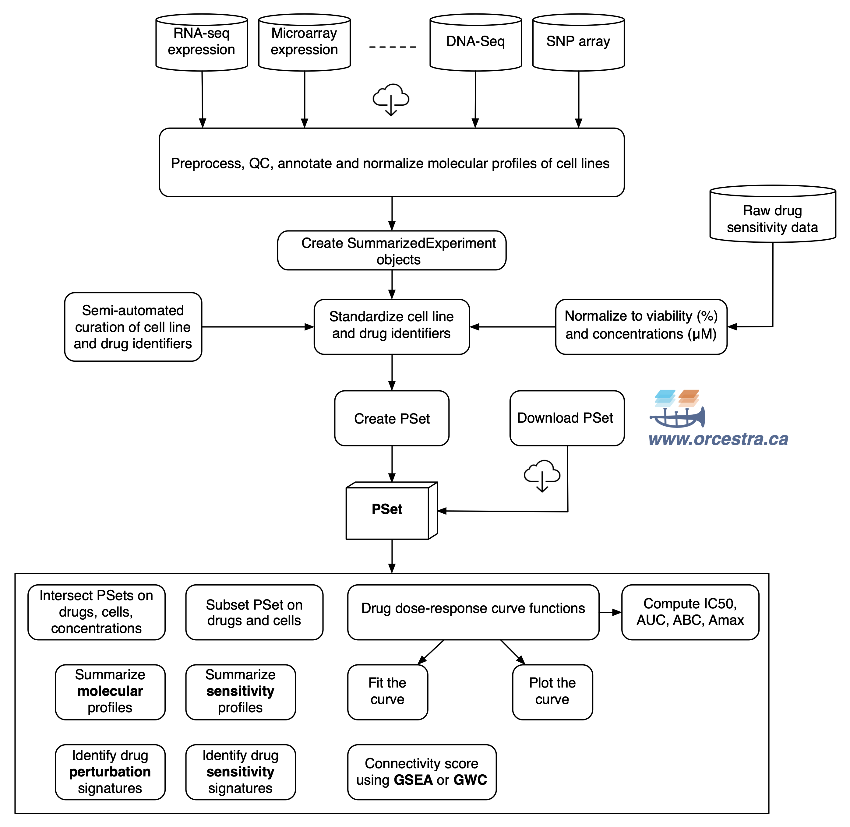
Drug sensitivity datasets refer to pharmacogenomic data where cancer cells are molecularly profiled at baseline (before drug treatment), and the effect of drug treatment on cell viability is measured using a pharmacological assay (e.g., Cell Titer-Glo). These datasets can be used for biomarker discovery by correlating the molecular features of cancer cells to their response to drugs of interest.

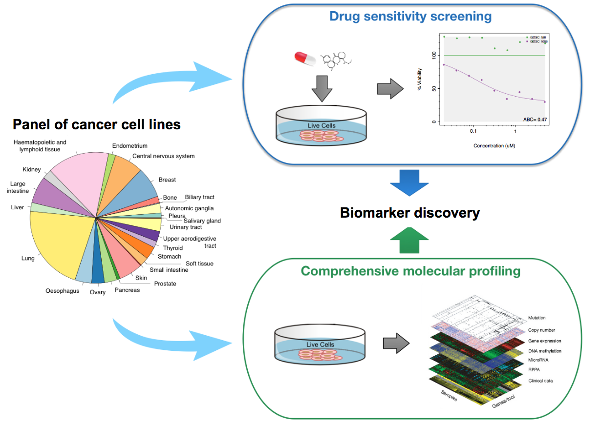
Schematic view of the drug sensitivity datasets.

Notably, the Genomics of Drug Sensitivity in Cancer GDSC and the Cancer Cell Line Encyclopedia CCLE are large drug sensitivity datasets published in seminal studies in Nature, Garnett et al., https://www.nature.com/articles/nature11005, Nature (2012) and Barretina et al., The Cancer Cell Line Encyclopedia enables predictive modelling of anticancer drug sensitivity, Nature (2012), respectively.

Drug Perturbation Datasets

Drug perturbation datasets refer to pharmacogenomic data where gene expression profiles are measured before and after short-term or medium term (e.g., 6h, 24h) drug treatment to identify genes that are up- and down-regulated due to the drug treatment. These datasets can be to classify drug (drug taxonomy), infer their mechanism of action, or find drugs with similar effects (drug repurposing).

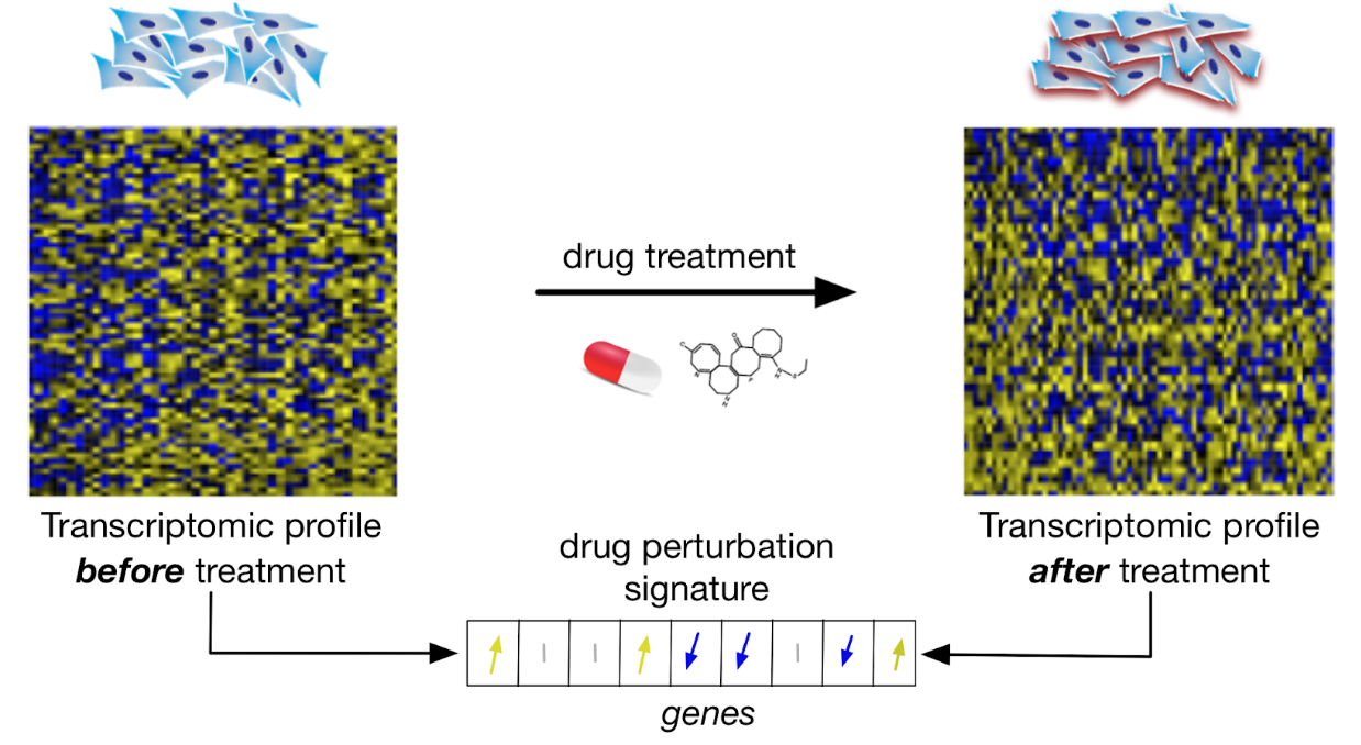
Schematic view of drug perturbation datasets

Large drug perturbation data have been generated within the Connectivity Map Project CAMP, with CMAPv2 and CMAPv3 available from PharmacoGx, published in Lamb et al., The Connectivity Map: Using Gene-Expression Signatures to Connect Small Molecules, Genes, and Disease, Science (2006) and Subramanian et al., A Next Generation Connectivity Map: L1000 Platform and the First 1,000,000 Profiles, Cell (2017), respectively.

Exploring Other Treatment Types

In addition to PharmacoGx, there is a suite of packages in Bioconductor for exploring public high throughput screening data. For Sensitivity datasets, Xeva provides access to public drug screening datasets in Patient Derived Xenograft models, including providing access to the Novartis PDX Encyclopedia dataset, published in Gao, H. et al. High-throughput screening using patient-derived tumor xenografts to predict clinical trial drug response, Nature Medicine.. Additionally, RadioGx is currently available in the development branch of Bioconductor, providing access to cell line screening data for response to radiation treatment, featuring data from Yard, B. D. et al. A genetic basis for the variation in the vulnerability of cancer to DNA damage. Nature Communications 7, 11428 (2016)..

The Biomarker Discovery from High Throughput Screening Datasets workshop at Bioc2020 goes into depth about using these packages for accessing and exploring public sensitivity datasets.

In addition, Bioconductor also includes the ToxicoGx package, which provides access to Sensitivity and Perturbation datasets characterizing in vitro response of human tissue to toxicant exposure, currently providing access to data from the TGGates and DrugMatrix datasets. More information about the ToxicoGx package can be found at the Bioc2020 poster presentation on the package.

Levi Waldron

Accessing The Cancer Genome Atlas (TCGA)

We summarize two approaches to accessing TCGA data:

1. TCGAbiolinks:
   1. data access through GenomicDataCommons
   2. provides data both from the legacy Firehose pipeline used by the TCGA publications (alignments based on hg18 and hg19 builds²), and the GDC harmonized GRCh38 pipeline³.
   3. downloads files from the Genomic Data Commons, and provides conversion to (Ranged)SummarizedExperiment where possible
2. curatedTCGAData:
   1. data access through ExperimentHub
   2. provides data from the legacy Firehose pipeline⁴
   3. provides individual assays as (Ranged)SummarizedExperiment and RaggedExperiment, integrates multiple assays within and across cancer types using MultiAssayExperiment

TCGAbiolinks

We demonstrate here generating a RangedSummarizedExperiment for RNA-seq data from adrenocortical carcinoma (ACC). For additional information and options, see the TCGAbiolinks vignettes⁵.

Load packages:

Search for matching data:

library(TCGAbiolinks)
library(SummarizedExperiment)
query <- GDCquery(project = "TCGA-ACC",
                           data.category = "Gene expression",
                           data.type = "Gene expression quantification",
                           platform = "Illumina HiSeq", 
                           file.type  = "normalized_results",
                           experimental.strategy = "RNA-Seq",
                           legacy = TRUE)

Download data and convert it to RangedSummarizedExperiment:

#gdcdir <- file.path("Waldron_PublicData", "GDCdata")
#GDCdownload(query, method = "api", files.per.chunk = 10,
#            directory = gdcdir)
#ACCse <- GDCprepare(query, directory = gdcdir)
#ACCse

curatedTCGAData: Curated Data From The Cancer Genome Atlas as MultiAssayExperiment Objects

curatedTCGAData does not interface with the Genomic Data Commons, but downloads data from Bioconductor’s ExperimentHub.

References: * https://waldronlab.io/MultiAssayWorkshop/articles/curatedTCGAData_ref.html : available datasets and data types. * https://waldronlab.io/MultiAssayWorkshop/articles/TCGAutilsCheatsheet.html : quick-reference for related utilities in TCGAutils package * https://waldronlab.io/MultiAssayWorkshop/articles/Ramos_MultiAssayExperiment.html: workshop for MultiAssayExperiment

library(curatedTCGAData)
library(MultiAssayExperiment)

By default, the curatedTCGAData() function will only show available datasets, and not download anything. The arguments are shown here only for demonstration, the same result is obtained with no arguments:

curatedTCGAData(diseaseCode = "*", assays = "*")

## using temporary cache /tmp/RtmpkiIQ1v/BiocFileCache

## snapshotDate(): 2020-10-27

## See '?curatedTCGAData' for 'diseaseCode' and 'assays' inputs

##      ah_id                                      title file_size
## 1    EH558                        ACC_CNASNP-20160128    0.8 Mb
## 2    EH559                        ACC_CNVSNP-20160128    0.2 Mb
## 3    EH561              ACC_GISTIC_AllByGene-20160128    0.3 Mb
## 4   EH2115                  ACC_GISTIC_Peaks-20160128      0 Mb
## 5    EH562      ACC_GISTIC_ThresholdedByGene-20160128    0.2 Mb
## 6   EH2116            ACC_Methylation-20160128_assays  236.4 Mb
## 7   EH2117                ACC_Methylation-20160128_se    6.1 Mb
## 8    EH565                  ACC_miRNASeqGene-20160128    0.1 Mb
## 9    EH566                      ACC_Mutation-20160128    0.7 Mb
## 10   EH567               ACC_RNASeq2GeneNorm-20160128      4 Mb
## 11   EH568                     ACC_RPPAArray-20160128    0.1 Mb
## 12   EH570                       BLCA_CNASeq-20160128    0.3 Mb
## 13   EH571                       BLCA_CNASNP-20160128    4.3 Mb
## 14   EH572                       BLCA_CNVSNP-20160128    1.1 Mb
## 15   EH574             BLCA_GISTIC_AllByGene-20160128    0.6 Mb
## 16  EH2118                 BLCA_GISTIC_Peaks-20160128      0 Mb
## 17   EH575     BLCA_GISTIC_ThresholdedByGene-20160128    0.3 Mb
## 18  EH2119           BLCA_Methylation-20160128_assays 1283.4 Mb
## 19  EH2120               BLCA_Methylation-20160128_se    6.1 Mb
## 20   EH578                 BLCA_miRNASeqGene-20160128    0.4 Mb
## 21   EH579                     BLCA_Mutation-20160128    3.7 Mb
## 22   EH580              BLCA_RNASeq2GeneNorm-20160128   21.9 Mb
## 23   EH581                   BLCA_RNASeqGene-20160128    2.4 Mb
## 24   EH582                    BLCA_RPPAArray-20160128    0.5 Mb
## 25   EH584                       BRCA_CNASeq-20160128      0 Mb
## 26   EH585                       BRCA_CNASNP-20160128    9.8 Mb
## 27   EH586                       BRCA_CNVSNP-20160128    2.8 Mb
## 28   EH588             BRCA_GISTIC_AllByGene-20160128    1.3 Mb
## 29  EH2121                 BRCA_GISTIC_Peaks-20160128      0 Mb
## 30   EH589     BRCA_GISTIC_ThresholdedByGene-20160128    0.4 Mb
## 31  EH2122  BRCA_Methylation_methyl27-20160128_assays   63.2 Mb
## 32  EH2123      BRCA_Methylation_methyl27-20160128_se    0.4 Mb
## 33  EH2124 BRCA_Methylation_methyl450-20160128_assays 2613.2 Mb
## 34  EH2125     BRCA_Methylation_methyl450-20160128_se    6.1 Mb
## 35   EH593                 BRCA_miRNASeqGene-20160128    0.6 Mb
## 36   EH594                    BRCA_mRNAArray-20160128   27.3 Mb
## 37   EH595                     BRCA_Mutation-20160128    4.5 Mb
## 38   EH596              BRCA_RNASeq2GeneNorm-20160128   64.5 Mb
## 39   EH597                   BRCA_RNASeqGene-20160128     30 Mb
## 40   EH598                    BRCA_RPPAArray-20160128    1.6 Mb
## 41   EH600                       CESC_CNASeq-20160128    0.1 Mb
## 42   EH601                       CESC_CNASNP-20160128    2.3 Mb
## 43   EH602                       CESC_CNVSNP-20160128    0.6 Mb
## 44   EH604             CESC_GISTIC_AllByGene-20160128    0.5 Mb
## 45  EH2126                 CESC_GISTIC_Peaks-20160128      0 Mb
## 46   EH605     CESC_GISTIC_ThresholdedByGene-20160128    0.3 Mb
## 47  EH2127           CESC_Methylation-20160128_assays  921.2 Mb
## 48  EH2128               CESC_Methylation-20160128_se    6.1 Mb
## 49   EH608                 CESC_miRNASeqGene-20160128    0.3 Mb
## 50   EH609                     CESC_Mutation-20160128      2 Mb
## 51   EH610              CESC_RNASeq2GeneNorm-20160128   16.1 Mb
## 52   EH611                    CESC_RPPAArray-20160128    0.3 Mb
## 53   EH613                       CHOL_CNASNP-20160128    0.4 Mb
## 54   EH614                       CHOL_CNVSNP-20160128    0.1 Mb
## 55   EH616             CHOL_GISTIC_AllByGene-20160128    0.3 Mb
## 56  EH2129                 CHOL_GISTIC_Peaks-20160128      0 Mb
## 57   EH617     CHOL_GISTIC_ThresholdedByGene-20160128    0.2 Mb
## 58  EH2130           CHOL_Methylation-20160128_assays  132.1 Mb
## 59  EH2131               CHOL_Methylation-20160128_se    6.1 Mb
## 60   EH620                 CHOL_miRNASeqGene-20160128    0.1 Mb
## 61   EH621                     CHOL_Mutation-20160128    0.2 Mb
## 62   EH622              CHOL_RNASeq2GeneNorm-20160128    2.4 Mb
## 63   EH623                    CHOL_RPPAArray-20160128    0.1 Mb
## 64   EH625                       COAD_CNASeq-20160128    0.3 Mb
## 65   EH626                       COAD_CNASNP-20160128    3.9 Mb
## 66   EH627                       COAD_CNVSNP-20160128    0.9 Mb
## 67   EH629             COAD_GISTIC_AllByGene-20160128    0.5 Mb
## 68  EH2132                 COAD_GISTIC_Peaks-20160128      0 Mb
## 69   EH630     COAD_GISTIC_ThresholdedByGene-20160128    0.3 Mb
## 70  EH2133  COAD_Methylation_methyl27-20160128_assays   37.2 Mb
## 71  EH2134      COAD_Methylation_methyl27-20160128_se    0.4 Mb
## 72  EH2135 COAD_Methylation_methyl450-20160128_assays  983.8 Mb
## 73  EH2136     COAD_Methylation_methyl450-20160128_se    6.1 Mb
## 74   EH634                 COAD_miRNASeqGene-20160128    0.2 Mb
## 75   EH635                    COAD_mRNAArray-20160128    8.1 Mb
## 76   EH636                     COAD_Mutation-20160128    1.2 Mb
## 77   EH637              COAD_RNASeq2GeneNorm-20160128    8.8 Mb
## 78   EH638                   COAD_RNASeqGene-20160128    0.4 Mb
## 79   EH639                    COAD_RPPAArray-20160128    0.6 Mb
## 80   EH641                       DLBC_CNASNP-20160128    0.4 Mb
## 81   EH642                       DLBC_CNVSNP-20160128    0.1 Mb
## 82   EH644             DLBC_GISTIC_AllByGene-20160128    0.2 Mb
## 83  EH2137                 DLBC_GISTIC_Peaks-20160128      0 Mb
## 84   EH645     DLBC_GISTIC_ThresholdedByGene-20160128    0.2 Mb
## 85  EH2138           DLBC_Methylation-20160128_assays  141.8 Mb
## 86  EH2139               DLBC_Methylation-20160128_se    6.1 Mb
## 87   EH648                 DLBC_miRNASeqGene-20160128    0.1 Mb
## 88   EH649                     DLBC_Mutation-20160128    0.7 Mb
## 89   EH650              DLBC_RNASeq2GeneNorm-20160128    2.5 Mb
## 90   EH651                    DLBC_RPPAArray-20160128    0.1 Mb
## 91   EH653                       ESCA_CNASeq-20160128    0.2 Mb
## 92   EH654                       ESCA_CNASNP-20160128    1.8 Mb
## 93   EH655                       ESCA_CNVSNP-20160128    0.7 Mb
## 94   EH657             ESCA_GISTIC_AllByGene-20160128    0.5 Mb
## 95  EH2140                 ESCA_GISTIC_Peaks-20160128      0 Mb
## 96   EH658     ESCA_GISTIC_ThresholdedByGene-20160128    0.2 Mb
## 97  EH2141           ESCA_Methylation-20160128_assays  596.9 Mb
## 98  EH2142               ESCA_Methylation-20160128_se    6.1 Mb
## 99   EH661                 ESCA_miRNASeqGene-20160128    0.2 Mb
## 100  EH662                     ESCA_Mutation-20160128    2.8 Mb
## 101  EH663              ESCA_RNASeq2GeneNorm-20160128   10.8 Mb
## 102  EH664                   ESCA_RNASeqGene-20160128      8 Mb
## 103  EH665                    ESCA_RPPAArray-20160128    0.2 Mb
## 104  EH667            GBM_CNACGH_CGH_hg_244a-20160128    0.7 Mb
## 105  EH668     GBM_CNACGH_CGH_hg_415k_g4124a-20160128    0.5 Mb
## 106  EH669                        GBM_CNASNP-20160128    5.2 Mb
## 107  EH670                        GBM_CNVSNP-20160128    1.5 Mb
## 108  EH672              GBM_GISTIC_AllByGene-20160128    0.7 Mb
## 109 EH2143                  GBM_GISTIC_Peaks-20160128      0 Mb
## 110  EH673      GBM_GISTIC_ThresholdedByGene-20160128    0.3 Mb
## 111 EH2144   GBM_Methylation_methyl27-20160128_assays   52.4 Mb
## 112 EH2145       GBM_Methylation_methyl27-20160128_se    0.4 Mb
## 113 EH2146  GBM_Methylation_methyl450-20160128_assays  455.1 Mb
## 114 EH2147      GBM_Methylation_methyl450-20160128_se    6.1 Mb
## 115  EH677                    GBM_miRNAArray-20160128    2.1 Mb
## 116  EH678                  GBM_miRNASeqGene-20160128      0 Mb
## 117  EH679                GBM_mRNAArray_huex-20160128   56.3 Mb
## 118 EH2148         GBM_mRNAArray_TX_g4502a_1-20160128   22.5 Mb
## 119  EH680           GBM_mRNAArray_TX_g4502a-20160128    5.7 Mb
## 120  EH681      GBM_mRNAArray_TX_ht_hg_u133a-20160128   44.7 Mb
## 121  EH682                      GBM_Mutation-20160128    2.1 Mb
## 122  EH683               GBM_RNASeq2GeneNorm-20160128    8.6 Mb
## 123  EH684                     GBM_RPPAArray-20160128    0.4 Mb
## 124  EH686                       HNSC_CNASeq-20160128    0.3 Mb
## 125  EH687                       HNSC_CNASNP-20160128    4.2 Mb
## 126  EH688                       HNSC_CNVSNP-20160128    1.1 Mb
## 127  EH690             HNSC_GISTIC_AllByGene-20160128    0.6 Mb
## 128 EH2149                 HNSC_GISTIC_Peaks-20160128      0 Mb
## 129  EH691     HNSC_GISTIC_ThresholdedByGene-20160128    0.3 Mb
## 130 EH2150           HNSC_Methylation-20160128_assays 1714.7 Mb
## 131 EH2151               HNSC_Methylation-20160128_se    6.1 Mb
## 132  EH694                 HNSC_miRNASeqGene-20160128    0.4 Mb
## 133  EH695                     HNSC_Mutation-20160128    4.8 Mb
## 134  EH696              HNSC_RNASeq2GeneNorm-20160128   29.5 Mb
## 135  EH697                   HNSC_RNASeqGene-20160128   10.3 Mb
## 136  EH698                    HNSC_RPPAArray-20160128    0.3 Mb
## 137  EH700                       KICH_CNASNP-20160128    0.5 Mb
## 138  EH701                       KICH_CNVSNP-20160128    0.1 Mb
## 139  EH703             KICH_GISTIC_AllByGene-20160128    0.2 Mb
## 140 EH2152                 KICH_GISTIC_Peaks-20160128      0 Mb
## 141  EH704     KICH_GISTIC_ThresholdedByGene-20160128    0.2 Mb
## 142 EH2153           KICH_Methylation-20160128_assays    195 Mb
## 143 EH2154               KICH_Methylation-20160128_se    6.1 Mb
## 144  EH707                 KICH_miRNASeqGene-20160128    0.1 Mb
## 145  EH708                     KICH_Mutation-20160128    0.1 Mb
## 146  EH709              KICH_RNASeq2GeneNorm-20160128    4.9 Mb
## 147  EH710                    KICH_RPPAArray-20160128    0.1 Mb
## 148  EH712                       KIRC_CNASNP-20160128    4.1 Mb
## 149  EH713                       KIRC_CNVSNP-20160128    0.8 Mb
## 150  EH715             KIRC_GISTIC_AllByGene-20160128    0.5 Mb
## 151 EH2155                 KIRC_GISTIC_Peaks-20160128      0 Mb
## 152  EH716     KIRC_GISTIC_ThresholdedByGene-20160128    0.2 Mb
## 153 EH2156  KIRC_Methylation_methyl27-20160128_assays   76.8 Mb
## 154 EH2157      KIRC_Methylation_methyl27-20160128_se    0.4 Mb
## 155 EH2158 KIRC_Methylation_methyl450-20160128_assays 1418.8 Mb
## 156 EH2159     KIRC_Methylation_methyl450-20160128_se    6.1 Mb
## 157  EH720                 KIRC_miRNASeqGene-20160128    0.2 Mb
## 158  EH721                    KIRC_mRNAArray-20160128    3.5 Mb
## 159  EH722                     KIRC_Mutation-20160128    0.4 Mb
## 160  EH723              KIRC_RNASeq2GeneNorm-20160128   32.2 Mb
## 161  EH724                   KIRC_RNASeqGene-20160128   18.2 Mb
## 162  EH725                    KIRC_RPPAArray-20160128    0.8 Mb
## 163  EH727                       KIRP_CNASNP-20160128    2.6 Mb
## 164  EH728                       KIRP_CNVSNP-20160128    0.5 Mb
## 165  EH730             KIRP_GISTIC_AllByGene-20160128    0.3 Mb
## 166 EH2160                 KIRP_GISTIC_Peaks-20160128      0 Mb
## 167  EH731     KIRP_GISTIC_ThresholdedByGene-20160128    0.2 Mb
## 168 EH2161  KIRP_Methylation_methyl27-20160128_assays    3.9 Mb
## 169 EH2162      KIRP_Methylation_methyl27-20160128_se    0.4 Mb
## 170 EH2163 KIRP_Methylation_methyl450-20160128_assays    948 Mb
## 171 EH2164     KIRP_Methylation_methyl450-20160128_se    6.1 Mb
## 172  EH735                 KIRP_miRNASeqGene-20160128    0.3 Mb
## 173  EH736                    KIRP_mRNAArray-20160128    0.9 Mb
## 174  EH737                     KIRP_Mutation-20160128    0.5 Mb
## 175  EH738              KIRP_RNASeq2GeneNorm-20160128   16.7 Mb
## 176  EH739                   KIRP_RNASeqGene-20160128    0.6 Mb
## 177  EH740                    KIRP_RPPAArray-20160128    0.3 Mb
## 178  EH742                       LAML_CNASNP-20160128    7.6 Mb
## 179  EH743                       LAML_CNVSNP-20160128    0.3 Mb
## 180 EH2538             LAML_GISTIC_AllByGene-20160128    0.3 Mb
## 181 EH2539                 LAML_GISTIC_Peaks-20160128      0 Mb
## 182 EH2540     LAML_GISTIC_ThresholdedByGene-20160128    0.2 Mb
## 183 EH2166  LAML_Methylation_methyl27-20160128_assays   35.6 Mb
## 184 EH2167      LAML_Methylation_methyl27-20160128_se    0.4 Mb
## 185 EH2168 LAML_Methylation_methyl450-20160128_assays  572.8 Mb
## 186 EH2169     LAML_Methylation_methyl450-20160128_se    6.1 Mb
## 187  EH748                     LAML_Mutation-20160128    0.2 Mb
## 188  EH749              LAML_RNASeq2GeneNorm-20160128    8.1 Mb
## 189  EH750                   LAML_RNASeqGene-20160128    5.4 Mb
## 190  EH752                        LGG_CNASeq-20160128    0.1 Mb
## 191  EH753                        LGG_CNASNP-20160128    3.3 Mb
## 192  EH754                        LGG_CNVSNP-20160128    0.8 Mb
## 193  EH756              LGG_GISTIC_AllByGene-20160128    0.5 Mb
## 194 EH2170                  LGG_GISTIC_Peaks-20160128      0 Mb
## 195  EH757      LGG_GISTIC_ThresholdedByGene-20160128    0.2 Mb
## 196 EH2171            LGG_Methylation-20160128_assays 1564.1 Mb
## 197 EH2172                LGG_Methylation-20160128_se    6.1 Mb
## 198  EH760                  LGG_miRNASeqGene-20160128    0.4 Mb
## 199  EH761                     LGG_mRNAArray-20160128    1.7 Mb
## 200  EH762                      LGG_Mutation-20160128    0.2 Mb
## 201  EH763               LGG_RNASeq2GeneNorm-20160128   28.3 Mb
## 202  EH764                     LGG_RPPAArray-20160128    0.6 Mb
## 203  EH766                       LIHC_CNASNP-20160128    3.1 Mb
## 204  EH767                       LIHC_CNVSNP-20160128      1 Mb
## 205  EH769             LIHC_GISTIC_AllByGene-20160128    0.6 Mb
## 206 EH2173                 LIHC_GISTIC_Peaks-20160128      0 Mb
## 207  EH770     LIHC_GISTIC_ThresholdedByGene-20160128    0.3 Mb
## 208 EH2174           LIHC_Methylation-20160128_assays 1267.8 Mb
## 209 EH2175               LIHC_Methylation-20160128_se    6.1 Mb
## 210  EH773                 LIHC_miRNASeqGene-20160128    0.3 Mb
## 211  EH774                     LIHC_Mutation-20160128    0.9 Mb
## 212  EH775              LIHC_RNASeq2GeneNorm-20160128   20.6 Mb
## 213  EH776                   LIHC_RNASeqGene-20160128    0.9 Mb
## 214  EH777                    LIHC_RPPAArray-20160128    0.3 Mb
## 215  EH779                       LUAD_CNASeq-20160128    3.8 Mb
## 216  EH780                       LUAD_CNASNP-20160128    4.2 Mb
## 217  EH781                       LUAD_CNVSNP-20160128    1.2 Mb
## 218  EH783             LUAD_GISTIC_AllByGene-20160128    0.7 Mb
## 219 EH2176                 LUAD_GISTIC_Peaks-20160128      0 Mb
## 220  EH784     LUAD_GISTIC_ThresholdedByGene-20160128    0.3 Mb
## 221 EH2177  LUAD_Methylation_methyl27-20160128_assays   16.4 Mb
## 222 EH2178      LUAD_Methylation_methyl27-20160128_se    0.4 Mb
## 223 EH2179 LUAD_Methylation_methyl450-20160128_assays 1452.7 Mb
## 224 EH2180     LUAD_Methylation_methyl450-20160128_se    6.1 Mb
## 225  EH788                 LUAD_miRNASeqGene-20160128    0.4 Mb
## 226  EH789                    LUAD_mRNAArray-20160128    1.6 Mb
## 227  EH790                     LUAD_Mutation-20160128    6.7 Mb
## 228  EH791              LUAD_RNASeq2GeneNorm-20160128   29.8 Mb
## 229  EH792                   LUAD_RNASeqGene-20160128    5.6 Mb
## 230  EH793                    LUAD_RPPAArray-20160128    0.6 Mb
## 231  EH795                       LUSC_CNACGH-20160128    0.7 Mb
## 232  EH796                       LUSC_CNASNP-20160128    4.7 Mb
## 233  EH797                       LUSC_CNVSNP-20160128    1.4 Mb
## 234  EH799             LUSC_GISTIC_AllByGene-20160128    0.7 Mb
## 235 EH2181                 LUSC_GISTIC_Peaks-20160128      0 Mb
## 236  EH800     LUSC_GISTIC_ThresholdedByGene-20160128    0.3 Mb
## 237 EH2182  LUSC_Methylation_methyl27-20160128_assays   29.5 Mb
## 238 EH2183      LUSC_Methylation_methyl27-20160128_se    0.4 Mb
## 239 EH2184 LUSC_Methylation_methyl450-20160128_assays 1218.4 Mb
## 240 EH2185     LUSC_Methylation_methyl450-20160128_se    6.1 Mb
## 241  EH804                 LUSC_miRNASeqGene-20160128    0.3 Mb
## 242  EH805               LUSC_mRNAArray_huex-20160128   14.8 Mb
## 243  EH806          LUSC_mRNAArray_TX_g4502a-20160128    7.2 Mb
## 244  EH807     LUSC_mRNAArray_TX_ht_hg_u133a-20160128   11.4 Mb
## 245  EH808                     LUSC_Mutation-20160128    5.7 Mb
## 246  EH809              LUSC_RNASeq2GeneNorm-20160128   29.2 Mb
## 247  EH810                   LUSC_RNASeqGene-20160128    8.4 Mb
## 248  EH811                    LUSC_RPPAArray-20160128    0.5 Mb
## 249  EH813                       MESO_CNASNP-20160128    0.8 Mb
## 250  EH814                       MESO_CNVSNP-20160128    0.2 Mb
## 251  EH816             MESO_GISTIC_AllByGene-20160128    0.3 Mb
## 252 EH2186                 MESO_GISTIC_Peaks-20160128      0 Mb
## 253  EH817     MESO_GISTIC_ThresholdedByGene-20160128    0.2 Mb
## 254 EH2187           MESO_Methylation-20160128_assays  257.2 Mb
## 255 EH2188               MESO_Methylation-20160128_se    6.1 Mb
## 256  EH820                 MESO_miRNASeqGene-20160128    0.1 Mb
## 257  EH821              MESO_RNASeq2GeneNorm-20160128    4.6 Mb
## 258  EH822                    MESO_RPPAArray-20160128    0.1 Mb
## 259  EH824             OV_CNACGH_CGH_hg_244a-20160128    1.1 Mb
## 260  EH825      OV_CNACGH_CGH_hg_415k_g4124a-20160128    2.2 Mb
## 261  EH826                         OV_CNASNP-20160128    8.2 Mb
## 262  EH827                         OV_CNVSNP-20160128    2.7 Mb
## 263  EH829               OV_GISTIC_AllByGene-20160128    1.2 Mb
## 264 EH2189                   OV_GISTIC_Peaks-20160128      0 Mb
## 265  EH830       OV_GISTIC_ThresholdedByGene-20160128    0.4 Mb
## 266 EH2190    OV_Methylation_methyl27-20160128_assays  108.7 Mb
## 267 EH2191        OV_Methylation_methyl27-20160128_se    0.4 Mb
## 268 EH2192   OV_Methylation_methyl450-20160128_assays   29.6 Mb
## 269 EH2193       OV_Methylation_methyl450-20160128_se    6.1 Mb
## 270  EH834                     OV_miRNAArray-20160128    3.2 Mb
## 271  EH835                   OV_miRNASeqGene-20160128    0.3 Mb
## 272  EH836                 OV_mRNAArray_huex-20160128   75.2 Mb
## 273 EH2194          OV_mRNAArray_TX_g4502a_1-20160128   25.2 Mb
## 274  EH837            OV_mRNAArray_TX_g4502a-20160128    1.9 Mb
## 275  EH838       OV_mRNAArray_TX_ht_hg_u133a-20160128   44.6 Mb
## 276  EH839                       OV_Mutation-20160128    0.5 Mb
## 277  EH840                OV_RNASeq2GeneNorm-20160128   16.7 Mb
## 278  EH841                     OV_RNASeqGene-20160128   10.4 Mb
## 279  EH842                      OV_RPPAArray-20160128    0.7 Mb
## 280  EH844                       PAAD_CNASNP-20160128    1.7 Mb
## 281  EH845                       PAAD_CNVSNP-20160128    0.4 Mb
## 282  EH847             PAAD_GISTIC_AllByGene-20160128    0.4 Mb
## 283 EH2195                 PAAD_GISTIC_Peaks-20160128      0 Mb
## 284  EH848     PAAD_GISTIC_ThresholdedByGene-20160128    0.2 Mb
## 285 EH2196           PAAD_Methylation-20160128_assays  575.8 Mb
## 286 EH2197               PAAD_Methylation-20160128_se    6.1 Mb
## 287  EH851                 PAAD_miRNASeqGene-20160128    0.2 Mb
## 288  EH852                     PAAD_Mutation-20160128    6.8 Mb
## 289  EH853              PAAD_RNASeq2GeneNorm-20160128    9.7 Mb
## 290  EH854                    PAAD_RPPAArray-20160128    0.2 Mb
## 291  EH856                       PCPG_CNASNP-20160128    2.6 Mb
## 292  EH857                       PCPG_CNVSNP-20160128    0.3 Mb
## 293  EH859             PCPG_GISTIC_AllByGene-20160128    0.3 Mb
## 294 EH2198                 PCPG_GISTIC_Peaks-20160128      0 Mb
## 295  EH860     PCPG_GISTIC_ThresholdedByGene-20160128    0.2 Mb
## 296 EH2199           PCPG_Methylation-20160128_assays  552.9 Mb
## 297 EH2200               PCPG_Methylation-20160128_se    6.1 Mb
## 298  EH863                 PCPG_miRNASeqGene-20160128    0.2 Mb
## 299  EH864                     PCPG_Mutation-20160128    0.6 Mb
## 300  EH865              PCPG_RNASeq2GeneNorm-20160128    9.6 Mb
## 301  EH866                    PCPG_RPPAArray-20160128    0.1 Mb
## 302  EH868                       PRAD_CNASeq-20160128    0.2 Mb
## 303  EH869                       PRAD_CNASNP-20160128    4.9 Mb
## 304  EH870                       PRAD_CNVSNP-20160128    1.2 Mb
## 305  EH872             PRAD_GISTIC_AllByGene-20160128    0.6 Mb
## 306 EH2201                 PRAD_GISTIC_Peaks-20160128      0 Mb
## 307  EH873     PRAD_GISTIC_ThresholdedByGene-20160128    0.2 Mb
## 308 EH2202           PRAD_Methylation-20160128_assays 1622.5 Mb
## 309 EH2203               PRAD_Methylation-20160128_se    6.1 Mb
## 310  EH876                 PRAD_miRNASeqGene-20160128    0.4 Mb
## 311  EH877                     PRAD_Mutation-20160128    1.4 Mb
## 312  EH878              PRAD_RNASeq2GeneNorm-20160128   28.9 Mb
## 313  EH879                    PRAD_RPPAArray-20160128    0.5 Mb
## 314  EH881                       READ_CNASeq-20160128    0.4 Mb
## 315  EH882                       READ_CNASNP-20160128    1.4 Mb
## 316  EH883                       READ_CNVSNP-20160128    0.4 Mb
## 317  EH885             READ_GISTIC_AllByGene-20160128    0.3 Mb
## 318 EH2204                 READ_GISTIC_Peaks-20160128      0 Mb
## 319  EH886     READ_GISTIC_ThresholdedByGene-20160128    0.2 Mb
## 320 EH2205  READ_Methylation_methyl27-20160128_assays   13.5 Mb
## 321 EH2206      READ_Methylation_methyl27-20160128_se    0.4 Mb
## 322 EH2207 READ_Methylation_methyl450-20160128_assays  313.3 Mb
## 323 EH2208     READ_Methylation_methyl450-20160128_se    6.1 Mb
## 324  EH890                 READ_miRNASeqGene-20160128    0.1 Mb
## 325  EH891                    READ_mRNAArray-20160128    3.5 Mb
## 326  EH892                     READ_Mutation-20160128    0.4 Mb
## 327  EH893              READ_RNASeq2GeneNorm-20160128    3.5 Mb
## 328  EH894                   READ_RNASeqGene-20160128    2.1 Mb
## 329  EH895                    READ_RPPAArray-20160128    0.2 Mb
## 330  EH897                       SARC_CNASNP-20160128    3.1 Mb
## 331  EH898                       SARC_CNVSNP-20160128    1.1 Mb
## 332  EH900             SARC_GISTIC_AllByGene-20160128    0.6 Mb
## 333 EH2209                 SARC_GISTIC_Peaks-20160128      0 Mb
## 334  EH901     SARC_GISTIC_ThresholdedByGene-20160128    0.3 Mb
## 335 EH2210           SARC_Methylation-20160128_assays  794.3 Mb
## 336 EH2211               SARC_Methylation-20160128_se    6.1 Mb
## 337  EH904                 SARC_miRNASeqGene-20160128    0.2 Mb
## 338  EH905                     SARC_Mutation-20160128    1.1 Mb
## 339  EH906              SARC_RNASeq2GeneNorm-20160128   13.6 Mb
## 340  EH907                    SARC_RPPAArray-20160128    0.3 Mb
## 341 EH1029                       SKCM_CNASeq-20160128    0.3 Mb
## 342 EH1030                       SKCM_CNASNP-20160128    3.8 Mb
## 343 EH1031                       SKCM_CNVSNP-20160128    1.1 Mb
## 344 EH2541             SKCM_GISTIC_AllByGene-20160128    0.5 Mb
## 345 EH2542                 SKCM_GISTIC_Peaks-20160128      0 Mb
## 346 EH2543     SKCM_GISTIC_ThresholdedByGene-20160128    0.2 Mb
## 347 EH2213           SKCM_Methylation-20160128_assays 1403.5 Mb
## 348 EH2214               SKCM_Methylation-20160128_se    6.1 Mb
## 349 EH1033                 SKCM_miRNASeqGene-20160128    0.4 Mb
## 350 EH1034                     SKCM_Mutation-20160128   26.7 Mb
## 351 EH1035              SKCM_RNASeq2GeneNorm-20160128   24.5 Mb
## 352 EH1036                    SKCM_RPPAArray-20160128    0.6 Mb
## 353  EH920                       STAD_CNASeq-20160128    0.3 Mb
## 354  EH921                       STAD_CNASNP-20160128    3.8 Mb
## 355  EH922                       STAD_CNVSNP-20160128    1.2 Mb
## 356  EH924             STAD_GISTIC_AllByGene-20160128    0.7 Mb
## 357 EH2215                 STAD_GISTIC_Peaks-20160128      0 Mb
## 358  EH925     STAD_GISTIC_ThresholdedByGene-20160128    0.3 Mb
## 359 EH2216  STAD_Methylation_methyl27-20160128_assays   13.5 Mb
## 360 EH2217      STAD_Methylation_methyl27-20160128_se    0.4 Mb
## 361 EH2218 STAD_Methylation_methyl450-20160128_assays 1172.9 Mb
## 362 EH2219     STAD_Methylation_methyl450-20160128_se    6.1 Mb
## 363  EH929                 STAD_miRNASeqGene-20160128    0.3 Mb
## 364  EH930                     STAD_Mutation-20160128   13.2 Mb
## 365  EH931              STAD_RNASeq2GeneNorm-20160128   23.9 Mb
## 366  EH932                   STAD_RNASeqGene-20160128    1.6 Mb
## 367  EH933                    STAD_RPPAArray-20160128    0.5 Mb
## 368  EH935                       TGCT_CNASNP-20160128    1.2 Mb
## 369  EH936                       TGCT_CNVSNP-20160128    0.3 Mb
## 370  EH938             TGCT_GISTIC_AllByGene-20160128    0.3 Mb
## 371 EH2220                 TGCT_GISTIC_Peaks-20160128      0 Mb
## 372  EH939     TGCT_GISTIC_ThresholdedByGene-20160128    0.2 Mb
## 373 EH2221           TGCT_Methylation-20160128_assays  411.3 Mb
## 374 EH2222               TGCT_Methylation-20160128_se    6.1 Mb
## 375  EH942                 TGCT_miRNASeqGene-20160128    0.2 Mb
## 376  EH943                     TGCT_Mutation-20160128    0.5 Mb
## 377  EH944              TGCT_RNASeq2GeneNorm-20160128    7.4 Mb
## 378  EH945                    TGCT_RPPAArray-20160128    0.2 Mb
## 379  EH947                       THCA_CNASeq-20160128      0 Mb
## 380  EH948                       THCA_CNASNP-20160128    3.1 Mb
## 381  EH949                       THCA_CNVSNP-20160128    0.5 Mb
## 382  EH951             THCA_GISTIC_AllByGene-20160128    0.3 Mb
## 383 EH2223                 THCA_GISTIC_Peaks-20160128      0 Mb
## 384  EH952     THCA_GISTIC_ThresholdedByGene-20160128    0.2 Mb
## 385 EH2224           THCA_Methylation-20160128_assays 1674.6 Mb
## 386 EH2225               THCA_Methylation-20160128_se    6.1 Mb
## 387  EH955                 THCA_miRNASeqGene-20160128    0.5 Mb
## 388  EH956                     THCA_Mutation-20160128    0.9 Mb
## 389  EH957              THCA_RNASeq2GeneNorm-20160128   30.1 Mb
## 390  EH958                   THCA_RNASeqGene-20160128    0.2 Mb
## 391  EH959                    THCA_RPPAArray-20160128    0.3 Mb
## 392  EH961                       THYM_CNASNP-20160128    0.9 Mb
## 393  EH962                       THYM_CNVSNP-20160128    0.2 Mb
## 394  EH964             THYM_GISTIC_AllByGene-20160128    0.2 Mb
## 395 EH2226                 THYM_GISTIC_Peaks-20160128      0 Mb
## 396  EH965     THYM_GISTIC_ThresholdedByGene-20160128    0.2 Mb
## 397 EH2227           THYM_Methylation-20160128_assays  372.2 Mb
## 398 EH2228               THYM_Methylation-20160128_se    6.1 Mb
## 399  EH968                 THYM_miRNASeqGene-20160128    0.1 Mb
## 400  EH969                     THYM_Mutation-20160128    0.2 Mb
## 401  EH970              THYM_RNASeq2GeneNorm-20160128    6.4 Mb
## 402  EH971                    THYM_RPPAArray-20160128    0.2 Mb
## 403  EH973                       UCEC_CNASeq-20160128    0.3 Mb
## 404  EH974                       UCEC_CNASNP-20160128    5.4 Mb
## 405  EH975                       UCEC_CNVSNP-20160128    1.3 Mb
## 406  EH977             UCEC_GISTIC_AllByGene-20160128    0.7 Mb
## 407 EH2229                 UCEC_GISTIC_Peaks-20160128      0 Mb
## 408  EH978     UCEC_GISTIC_ThresholdedByGene-20160128    0.3 Mb
## 409 EH2230  UCEC_Methylation_methyl27-20160128_assays   21.7 Mb
## 410 EH2231      UCEC_Methylation_methyl27-20160128_se    0.4 Mb
## 411 EH2232 UCEC_Methylation_methyl450-20160128_assays   1377 Mb
## 412 EH2233     UCEC_Methylation_methyl450-20160128_se    6.1 Mb
## 413  EH982                 UCEC_miRNASeqGene-20160128    0.4 Mb
## 414  EH983                    UCEC_mRNAArray-20160128    2.6 Mb
## 415  EH984                     UCEC_Mutation-20160128    4.6 Mb
## 416  EH985              UCEC_RNASeq2GeneNorm-20160128   18.4 Mb
## 417  EH986                   UCEC_RNASeqGene-20160128    7.7 Mb
## 418  EH987                    UCEC_RPPAArray-20160128    0.7 Mb
## 419  EH989                        UCS_CNASNP-20160128    0.5 Mb
## 420  EH990                        UCS_CNVSNP-20160128    0.2 Mb
## 421  EH992              UCS_GISTIC_AllByGene-20160128    0.3 Mb
## 422 EH2234                  UCS_GISTIC_Peaks-20160128      0 Mb
## 423  EH993      UCS_GISTIC_ThresholdedByGene-20160128    0.3 Mb
## 424 EH2235            UCS_Methylation-20160128_assays  168.3 Mb
## 425 EH2236                UCS_Methylation-20160128_se    6.1 Mb
## 426  EH996                  UCS_miRNASeqGene-20160128    0.1 Mb
## 427  EH997                      UCS_Mutation-20160128    1.2 Mb
## 428  EH998               UCS_RNASeq2GeneNorm-20160128    3.1 Mb
## 429  EH999                     UCS_RPPAArray-20160128    0.1 Mb
## 430 EH1001                        UVM_CNASeq-20160128    0.1 Mb
## 431 EH1002                        UVM_CNASNP-20160128    0.6 Mb
## 432 EH1003                        UVM_CNVSNP-20160128    0.1 Mb
## 433 EH1005              UVM_GISTIC_AllByGene-20160128    0.3 Mb
## 434 EH2237                  UVM_GISTIC_Peaks-20160128      0 Mb
## 435 EH1006      UVM_GISTIC_ThresholdedByGene-20160128    0.2 Mb
## 436 EH2238            UVM_Methylation-20160128_assays  236.4 Mb
## 437 EH2239                UVM_Methylation-20160128_se    6.1 Mb
## 438 EH1009                  UVM_miRNASeqGene-20160128    0.1 Mb
## 439 EH1010                      UVM_Mutation-20160128    0.9 Mb
## 440 EH1011               UVM_RNASeq2GeneNorm-20160128      4 Mb
## 441 EH1012                     UVM_RPPAArray-20160128      0 Mb
##                     rdataclass rdatadateadded rdatadateremoved
## 1             RaggedExperiment     2017-10-10             <NA>
## 2             RaggedExperiment     2017-10-10             <NA>
## 3         SummarizedExperiment     2017-10-10             <NA>
## 4   RangedSummarizedExperiment     2019-01-09             <NA>
## 5         SummarizedExperiment     2017-10-10             <NA>
## 6         SummarizedExperiment     2019-01-09             <NA>
## 7             RaggedExperiment     2019-01-09             <NA>
## 8         SummarizedExperiment     2017-10-10             <NA>
## 9             RaggedExperiment     2017-10-10             <NA>
## 10        SummarizedExperiment     2017-10-10             <NA>
## 11        SummarizedExperiment     2017-10-10             <NA>
## 12            RaggedExperiment     2017-10-10             <NA>
## 13            RaggedExperiment     2017-10-10             <NA>
## 14            RaggedExperiment     2017-10-10             <NA>
## 15        SummarizedExperiment     2017-10-10             <NA>
## 16  RangedSummarizedExperiment     2019-01-09             <NA>
## 17        SummarizedExperiment     2017-10-10             <NA>
## 18        SummarizedExperiment     2019-01-09             <NA>
## 19            RaggedExperiment     2019-01-09             <NA>
## 20        SummarizedExperiment     2017-10-10             <NA>
## 21            RaggedExperiment     2017-10-10             <NA>
## 22        SummarizedExperiment     2017-10-10             <NA>
## 23        SummarizedExperiment     2017-10-10             <NA>
## 24        SummarizedExperiment     2017-10-10             <NA>
## 25            RaggedExperiment     2017-10-10             <NA>
## 26            RaggedExperiment     2017-10-10             <NA>
## 27            RaggedExperiment     2017-10-10             <NA>
## 28        SummarizedExperiment     2017-10-10             <NA>
## 29  RangedSummarizedExperiment     2019-01-09             <NA>
## 30        SummarizedExperiment     2017-10-10             <NA>
## 31        SummarizedExperiment     2019-01-09             <NA>
## 32        SummarizedExperiment     2019-01-09             <NA>
## 33            RaggedExperiment     2019-01-09             <NA>
## 34        SummarizedExperiment     2019-01-09             <NA>
## 35        SummarizedExperiment     2017-10-10             <NA>
## 36        SummarizedExperiment     2017-10-10             <NA>
## 37            RaggedExperiment     2017-10-10             <NA>
## 38        SummarizedExperiment     2017-10-10             <NA>
## 39        SummarizedExperiment     2017-10-10             <NA>
## 40        SummarizedExperiment     2017-10-10             <NA>
## 41            RaggedExperiment     2017-10-10             <NA>
## 42            RaggedExperiment     2017-10-10             <NA>
## 43            RaggedExperiment     2017-10-10             <NA>
## 44        SummarizedExperiment     2017-10-10             <NA>
## 45  RangedSummarizedExperiment     2019-01-09             <NA>
## 46        SummarizedExperiment     2017-10-10             <NA>
## 47        SummarizedExperiment     2019-01-09             <NA>
## 48            RaggedExperiment     2019-01-09             <NA>
## 49        SummarizedExperiment     2017-10-10             <NA>
## 50            RaggedExperiment     2017-10-10             <NA>
## 51        SummarizedExperiment     2017-10-10             <NA>
## 52        SummarizedExperiment     2017-10-10             <NA>
## 53            RaggedExperiment     2017-10-10             <NA>
## 54            RaggedExperiment     2017-10-10             <NA>
## 55        SummarizedExperiment     2017-10-10             <NA>
## 56  RangedSummarizedExperiment     2019-01-09             <NA>
## 57        SummarizedExperiment     2017-10-10             <NA>
## 58        SummarizedExperiment     2019-01-09             <NA>
## 59            RaggedExperiment     2019-01-09             <NA>
## 60        SummarizedExperiment     2017-10-10             <NA>
## 61            RaggedExperiment     2017-10-10             <NA>
## 62        SummarizedExperiment     2017-10-10             <NA>
## 63        SummarizedExperiment     2017-10-10             <NA>
## 64            RaggedExperiment     2017-10-10             <NA>
## 65            RaggedExperiment     2017-10-10             <NA>
## 66            RaggedExperiment     2017-10-10             <NA>
## 67        SummarizedExperiment     2017-10-10             <NA>
## 68  RangedSummarizedExperiment     2019-01-09             <NA>
## 69        SummarizedExperiment     2017-10-10             <NA>
## 70        SummarizedExperiment     2019-01-09             <NA>
## 71        SummarizedExperiment     2019-01-09             <NA>
## 72            RaggedExperiment     2019-01-09             <NA>
## 73        SummarizedExperiment     2019-01-09             <NA>
## 74        SummarizedExperiment     2017-10-10             <NA>
## 75        SummarizedExperiment     2017-10-10             <NA>
## 76            RaggedExperiment     2017-10-10             <NA>
## 77        SummarizedExperiment     2017-10-10             <NA>
## 78        SummarizedExperiment     2017-10-10             <NA>
## 79        SummarizedExperiment     2017-10-10             <NA>
## 80            RaggedExperiment     2017-10-10             <NA>
## 81            RaggedExperiment     2017-10-10             <NA>
## 82        SummarizedExperiment     2017-10-10             <NA>
## 83  RangedSummarizedExperiment     2019-01-09             <NA>
## 84        SummarizedExperiment     2017-10-10             <NA>
## 85        SummarizedExperiment     2019-01-09             <NA>
## 86            RaggedExperiment     2019-01-09             <NA>
## 87        SummarizedExperiment     2017-10-10             <NA>
## 88            RaggedExperiment     2017-10-10             <NA>
## 89        SummarizedExperiment     2017-10-10             <NA>
## 90        SummarizedExperiment     2017-10-10             <NA>
## 91            RaggedExperiment     2017-10-10             <NA>
## 92            RaggedExperiment     2017-10-10             <NA>
## 93            RaggedExperiment     2017-10-10             <NA>
## 94        SummarizedExperiment     2017-10-10             <NA>
## 95  RangedSummarizedExperiment     2019-01-09             <NA>
## 96        SummarizedExperiment     2017-10-10             <NA>
## 97        SummarizedExperiment     2019-01-09             <NA>
## 98            RaggedExperiment     2019-01-09             <NA>
## 99        SummarizedExperiment     2017-10-10             <NA>
## 100           RaggedExperiment     2017-10-10             <NA>
## 101       SummarizedExperiment     2017-10-10             <NA>
## 102       SummarizedExperiment     2017-10-10             <NA>
## 103       SummarizedExperiment     2017-10-10             <NA>
## 104           RaggedExperiment     2017-10-10             <NA>
## 105           RaggedExperiment     2017-10-10             <NA>
## 106           RaggedExperiment     2017-10-10             <NA>
## 107           RaggedExperiment     2017-10-10             <NA>
## 108       SummarizedExperiment     2017-10-10             <NA>
## 109 RangedSummarizedExperiment     2019-01-09             <NA>
## 110       SummarizedExperiment     2017-10-10             <NA>
## 111       SummarizedExperiment     2019-01-09             <NA>
## 112       SummarizedExperiment     2019-01-09             <NA>
## 113       SummarizedExperiment     2019-01-09             <NA>
## 114       SummarizedExperiment     2019-01-09             <NA>
## 115       SummarizedExperiment     2017-10-10             <NA>
## 116       SummarizedExperiment     2017-10-10             <NA>
## 117       SummarizedExperiment     2017-10-10             <NA>
## 118       SummarizedExperiment     2019-01-09             <NA>
## 119       SummarizedExperiment     2017-10-10             <NA>
## 120       SummarizedExperiment     2017-10-10             <NA>
## 121           RaggedExperiment     2017-10-10             <NA>
## 122       SummarizedExperiment     2017-10-10             <NA>
## 123       SummarizedExperiment     2017-10-10             <NA>
## 124           RaggedExperiment     2017-10-10             <NA>
## 125           RaggedExperiment     2017-10-10             <NA>
## 126           RaggedExperiment     2017-10-10             <NA>
## 127       SummarizedExperiment     2017-10-10             <NA>
## 128 RangedSummarizedExperiment     2019-01-09             <NA>
## 129       SummarizedExperiment     2017-10-10             <NA>
## 130       SummarizedExperiment     2019-01-09             <NA>
## 131           RaggedExperiment     2019-01-09             <NA>
## 132       SummarizedExperiment     2017-10-10             <NA>
## 133           RaggedExperiment     2017-10-10             <NA>
## 134       SummarizedExperiment     2017-10-10             <NA>
## 135       SummarizedExperiment     2017-10-10             <NA>
## 136       SummarizedExperiment     2017-10-10             <NA>
## 137           RaggedExperiment     2017-10-10             <NA>
## 138           RaggedExperiment     2017-10-10             <NA>
## 139       SummarizedExperiment     2017-10-10             <NA>
## 140 RangedSummarizedExperiment     2019-01-09             <NA>
## 141       SummarizedExperiment     2017-10-10             <NA>
## 142       SummarizedExperiment     2019-01-09             <NA>
## 143           RaggedExperiment     2019-01-09             <NA>
## 144       SummarizedExperiment     2017-10-10             <NA>
## 145           RaggedExperiment     2017-10-10             <NA>
## 146       SummarizedExperiment     2017-10-10             <NA>
## 147       SummarizedExperiment     2017-10-10             <NA>
## 148           RaggedExperiment     2017-10-10             <NA>
## 149           RaggedExperiment     2017-10-10             <NA>
## 150       SummarizedExperiment     2017-10-10             <NA>
## 151 RangedSummarizedExperiment     2019-01-09             <NA>
## 152       SummarizedExperiment     2017-10-10             <NA>
## 153       SummarizedExperiment     2019-01-09             <NA>
## 154       SummarizedExperiment     2019-01-09             <NA>
## 155           RaggedExperiment     2019-01-09             <NA>
## 156       SummarizedExperiment     2019-01-09             <NA>
## 157       SummarizedExperiment     2017-10-10             <NA>
## 158       SummarizedExperiment     2017-10-10             <NA>
## 159           RaggedExperiment     2017-10-10             <NA>
## 160       SummarizedExperiment     2017-10-10             <NA>
## 161       SummarizedExperiment     2017-10-10             <NA>
## 162       SummarizedExperiment     2017-10-10             <NA>
## 163           RaggedExperiment     2017-10-10             <NA>
## 164           RaggedExperiment     2017-10-10             <NA>
## 165       SummarizedExperiment     2017-10-10             <NA>
## 166 RangedSummarizedExperiment     2019-01-09             <NA>
## 167       SummarizedExperiment     2017-10-10             <NA>
## 168       SummarizedExperiment     2019-01-09             <NA>
## 169       SummarizedExperiment     2019-01-09             <NA>
## 170           RaggedExperiment     2019-01-09             <NA>
## 171       SummarizedExperiment     2019-01-09             <NA>
## 172       SummarizedExperiment     2017-10-10             <NA>
## 173       SummarizedExperiment     2017-10-10             <NA>
## 174           RaggedExperiment     2017-10-10             <NA>
## 175       SummarizedExperiment     2017-10-10             <NA>
## 176       SummarizedExperiment     2017-10-10             <NA>
## 177       SummarizedExperiment     2017-10-10             <NA>
## 178           RaggedExperiment     2017-10-10             <NA>
## 179           RaggedExperiment     2017-10-10             <NA>
## 180       SummarizedExperiment     2019-04-29             <NA>
## 181 RangedSummarizedExperiment     2019-04-29             <NA>
## 182       SummarizedExperiment     2019-04-29             <NA>
## 183           RaggedExperiment     2019-01-09             <NA>
## 184       SummarizedExperiment     2019-01-09             <NA>
## 185       SummarizedExperiment     2019-01-09             <NA>
## 186                  DataFrame     2019-01-09             <NA>
## 187           RaggedExperiment     2017-10-10             <NA>
## 188       SummarizedExperiment     2017-10-10             <NA>
## 189       SummarizedExperiment     2017-10-10             <NA>
## 190           RaggedExperiment     2017-10-10             <NA>
## 191           RaggedExperiment     2017-10-10             <NA>
## 192           RaggedExperiment     2017-10-10             <NA>
## 193       SummarizedExperiment     2017-10-10             <NA>
## 194 RangedSummarizedExperiment     2019-01-09             <NA>
## 195       SummarizedExperiment     2017-10-10             <NA>
## 196       SummarizedExperiment     2019-01-09             <NA>
## 197       SummarizedExperiment     2019-01-09             <NA>
## 198       SummarizedExperiment     2017-10-10             <NA>
## 199       SummarizedExperiment     2017-10-10             <NA>
## 200           RaggedExperiment     2017-10-10             <NA>
## 201       SummarizedExperiment     2017-10-10             <NA>
## 202       SummarizedExperiment     2017-10-10             <NA>
## 203           RaggedExperiment     2017-10-10             <NA>
## 204           RaggedExperiment     2017-10-10             <NA>
## 205       SummarizedExperiment     2017-10-10             <NA>
## 206 RangedSummarizedExperiment     2019-01-09             <NA>
## 207       SummarizedExperiment     2017-10-10             <NA>
## 208       SummarizedExperiment     2019-01-09             <NA>
## 209           RaggedExperiment     2019-01-09             <NA>
## 210       SummarizedExperiment     2017-10-10             <NA>
## 211           RaggedExperiment     2017-10-10             <NA>
## 212       SummarizedExperiment     2017-10-10             <NA>
## 213       SummarizedExperiment     2017-10-10             <NA>
## 214       SummarizedExperiment     2017-10-10             <NA>
## 215           RaggedExperiment     2017-10-10             <NA>
## 216           RaggedExperiment     2017-10-10             <NA>
## 217           RaggedExperiment     2017-10-10             <NA>
## 218       SummarizedExperiment     2017-10-10             <NA>
## 219 RangedSummarizedExperiment     2019-01-09             <NA>
## 220       SummarizedExperiment     2017-10-10             <NA>
## 221       SummarizedExperiment     2019-01-09             <NA>
## 222       SummarizedExperiment     2019-01-09             <NA>
## 223           RaggedExperiment     2019-01-09             <NA>
## 224       SummarizedExperiment     2019-01-09             <NA>
## 225       SummarizedExperiment     2017-10-10             <NA>
## 226       SummarizedExperiment     2017-10-10             <NA>
## 227           RaggedExperiment     2017-10-10             <NA>
## 228       SummarizedExperiment     2017-10-10             <NA>
## 229       SummarizedExperiment     2017-10-10             <NA>
## 230       SummarizedExperiment     2017-10-10             <NA>
## 231           RaggedExperiment     2017-10-10             <NA>
## 232           RaggedExperiment     2017-10-10             <NA>
## 233           RaggedExperiment     2017-10-10             <NA>
## 234       SummarizedExperiment     2017-10-10             <NA>
## 235 RangedSummarizedExperiment     2019-01-09             <NA>
## 236       SummarizedExperiment     2017-10-10             <NA>
## 237       SummarizedExperiment     2019-01-09             <NA>
## 238       SummarizedExperiment     2019-01-09             <NA>
## 239       SummarizedExperiment     2019-01-09             <NA>
## 240       SummarizedExperiment     2019-01-09             <NA>
## 241       SummarizedExperiment     2017-10-10             <NA>
## 242       SummarizedExperiment     2017-10-10             <NA>
## 243       SummarizedExperiment     2017-10-10             <NA>
## 244       SummarizedExperiment     2017-10-10             <NA>
## 245           RaggedExperiment     2017-10-10             <NA>
## 246       SummarizedExperiment     2017-10-10             <NA>
## 247       SummarizedExperiment     2017-10-10             <NA>
## 248       SummarizedExperiment     2017-10-10             <NA>
## 249           RaggedExperiment     2017-10-10             <NA>
## 250           RaggedExperiment     2017-10-10             <NA>
## 251       SummarizedExperiment     2017-10-10             <NA>
## 252 RangedSummarizedExperiment     2019-01-09             <NA>
## 253       SummarizedExperiment     2017-10-10             <NA>
## 254       SummarizedExperiment     2019-01-09             <NA>
## 255       SummarizedExperiment     2019-01-09             <NA>
## 256       SummarizedExperiment     2017-10-10             <NA>
## 257       SummarizedExperiment     2017-10-10             <NA>
## 258       SummarizedExperiment     2017-10-10             <NA>
## 259           RaggedExperiment     2017-10-10             <NA>
## 260           RaggedExperiment     2017-10-10             <NA>
## 261           RaggedExperiment     2017-10-10             <NA>
## 262           RaggedExperiment     2017-10-10             <NA>
## 263       SummarizedExperiment     2017-10-10             <NA>
## 264 RangedSummarizedExperiment     2019-01-09             <NA>
## 265       SummarizedExperiment     2017-10-10             <NA>
## 266       SummarizedExperiment     2019-01-09             <NA>
## 267       SummarizedExperiment     2019-01-09             <NA>
## 268       SummarizedExperiment     2019-01-09             <NA>
## 269       SummarizedExperiment     2019-01-09             <NA>
## 270       SummarizedExperiment     2017-10-10             <NA>
## 271       SummarizedExperiment     2017-10-10             <NA>
## 272       SummarizedExperiment     2017-10-10             <NA>
## 273       SummarizedExperiment     2019-01-09             <NA>
## 274       SummarizedExperiment     2017-10-10             <NA>
## 275       SummarizedExperiment     2017-10-10             <NA>
## 276           RaggedExperiment     2017-10-10             <NA>
## 277       SummarizedExperiment     2017-10-10             <NA>
## 278       SummarizedExperiment     2017-10-10             <NA>
## 279       SummarizedExperiment     2017-10-10             <NA>
## 280           RaggedExperiment     2017-10-10             <NA>
## 281           RaggedExperiment     2017-10-10             <NA>
## 282       SummarizedExperiment     2017-10-10             <NA>
## 283 RangedSummarizedExperiment     2019-01-09             <NA>
## 284       SummarizedExperiment     2017-10-10             <NA>
## 285       SummarizedExperiment     2019-01-09             <NA>
## 286           RaggedExperiment     2019-01-09             <NA>
## 287       SummarizedExperiment     2017-10-10             <NA>
## 288           RaggedExperiment     2017-10-10             <NA>
## 289       SummarizedExperiment     2017-10-10             <NA>
## 290       SummarizedExperiment     2017-10-10             <NA>
## 291           RaggedExperiment     2017-10-10             <NA>
## 292           RaggedExperiment     2017-10-10             <NA>
## 293       SummarizedExperiment     2017-10-10             <NA>
## 294 RangedSummarizedExperiment     2019-01-09             <NA>
## 295       SummarizedExperiment     2017-10-10             <NA>
## 296       SummarizedExperiment     2019-01-09             <NA>
## 297           RaggedExperiment     2019-01-09             <NA>
## 298       SummarizedExperiment     2017-10-10             <NA>
## 299           RaggedExperiment     2017-10-10             <NA>
## 300       SummarizedExperiment     2017-10-10             <NA>
## 301       SummarizedExperiment     2017-10-10             <NA>
## 302           RaggedExperiment     2017-10-10             <NA>
## 303           RaggedExperiment     2017-10-10             <NA>
## 304           RaggedExperiment     2017-10-10             <NA>
## 305       SummarizedExperiment     2017-10-10             <NA>
## 306 RangedSummarizedExperiment     2019-01-09             <NA>
## 307       SummarizedExperiment     2017-10-10             <NA>
## 308       SummarizedExperiment     2019-01-09             <NA>
## 309           RaggedExperiment     2019-01-09             <NA>
## 310       SummarizedExperiment     2017-10-10             <NA>
## 311           RaggedExperiment     2017-10-10             <NA>
## 312       SummarizedExperiment     2017-10-10             <NA>
## 313       SummarizedExperiment     2017-10-10             <NA>
## 314           RaggedExperiment     2017-10-10             <NA>
## 315           RaggedExperiment     2017-10-10             <NA>
## 316           RaggedExperiment     2017-10-10             <NA>
## 317       SummarizedExperiment     2017-10-10             <NA>
## 318 RangedSummarizedExperiment     2019-01-09             <NA>
## 319       SummarizedExperiment     2017-10-10             <NA>
## 320       SummarizedExperiment     2019-01-09             <NA>
## 321       SummarizedExperiment     2019-01-09             <NA>
## 322           RaggedExperiment     2019-01-09             <NA>
## 323       SummarizedExperiment     2019-01-09             <NA>
## 324       SummarizedExperiment     2017-10-10             <NA>
## 325       SummarizedExperiment     2017-10-10             <NA>
## 326           RaggedExperiment     2017-10-10             <NA>
## 327       SummarizedExperiment     2017-10-10             <NA>
## 328       SummarizedExperiment     2017-10-10             <NA>
## 329       SummarizedExperiment     2017-10-10             <NA>
## 330           RaggedExperiment     2017-10-10             <NA>
## 331           RaggedExperiment     2017-10-10             <NA>
## 332       SummarizedExperiment     2017-10-10             <NA>
## 333 RangedSummarizedExperiment     2019-01-09             <NA>
## 334       SummarizedExperiment     2017-10-10             <NA>
## 335       SummarizedExperiment     2019-01-09             <NA>
## 336           RaggedExperiment     2019-01-09             <NA>
## 337       SummarizedExperiment     2017-10-10             <NA>
## 338           RaggedExperiment     2017-10-10             <NA>
## 339       SummarizedExperiment     2017-10-10             <NA>
## 340       SummarizedExperiment     2017-10-10             <NA>
## 341           RaggedExperiment     2017-10-16             <NA>
## 342           RaggedExperiment     2017-10-16             <NA>
## 343           RaggedExperiment     2017-10-16             <NA>
## 344       SummarizedExperiment     2019-04-29             <NA>
## 345 RangedSummarizedExperiment     2019-04-29             <NA>
## 346       SummarizedExperiment     2019-04-29             <NA>
## 347       SummarizedExperiment     2019-01-09             <NA>
## 348           RaggedExperiment     2019-01-09             <NA>
## 349       SummarizedExperiment     2017-10-16             <NA>
## 350           RaggedExperiment     2017-10-16             <NA>
## 351       SummarizedExperiment     2017-10-16             <NA>
## 352       SummarizedExperiment     2017-10-16             <NA>
## 353           RaggedExperiment     2017-10-10             <NA>
## 354           RaggedExperiment     2017-10-10             <NA>
## 355           RaggedExperiment     2017-10-10             <NA>
## 356       SummarizedExperiment     2017-10-10             <NA>
## 357 RangedSummarizedExperiment     2019-01-09             <NA>
## 358       SummarizedExperiment     2017-10-10             <NA>
## 359       SummarizedExperiment     2019-01-09             <NA>
## 360           RaggedExperiment     2019-01-09             <NA>
## 361       SummarizedExperiment     2019-01-09             <NA>
## 362       SummarizedExperiment     2019-01-09             <NA>
## 363       SummarizedExperiment     2017-10-10             <NA>
## 364           RaggedExperiment     2017-10-10             <NA>
## 365       SummarizedExperiment     2017-10-10             <NA>
## 366       SummarizedExperiment     2017-10-10             <NA>
## 367       SummarizedExperiment     2017-10-10             <NA>
## 368           RaggedExperiment     2017-10-10             <NA>
## 369           RaggedExperiment     2017-10-10             <NA>
## 370       SummarizedExperiment     2017-10-10             <NA>
## 371 RangedSummarizedExperiment     2019-01-09             <NA>
## 372       SummarizedExperiment     2017-10-10             <NA>
## 373       SummarizedExperiment     2019-01-09             <NA>
## 374           RaggedExperiment     2019-01-09             <NA>
## 375       SummarizedExperiment     2017-10-10             <NA>
## 376           RaggedExperiment     2017-10-10             <NA>
## 377       SummarizedExperiment     2017-10-10             <NA>
## 378       SummarizedExperiment     2017-10-10             <NA>
## 379           RaggedExperiment     2017-10-10             <NA>
## 380           RaggedExperiment     2017-10-10             <NA>
## 381           RaggedExperiment     2017-10-10             <NA>
## 382       SummarizedExperiment     2017-10-10             <NA>
## 383 RangedSummarizedExperiment     2019-01-09             <NA>
## 384       SummarizedExperiment     2017-10-10             <NA>
## 385       SummarizedExperiment     2019-01-09             <NA>
## 386           RaggedExperiment     2019-01-09             <NA>
## 387       SummarizedExperiment     2017-10-10             <NA>
## 388           RaggedExperiment     2017-10-10             <NA>
## 389       SummarizedExperiment     2017-10-10             <NA>
## 390       SummarizedExperiment     2017-10-10             <NA>
## 391       SummarizedExperiment     2017-10-10             <NA>
## 392           RaggedExperiment     2017-10-10             <NA>
## 393           RaggedExperiment     2017-10-10             <NA>
## 394       SummarizedExperiment     2017-10-10             <NA>
## 395 RangedSummarizedExperiment     2019-01-09             <NA>
## 396       SummarizedExperiment     2017-10-10             <NA>
## 397       SummarizedExperiment     2019-01-09             <NA>
## 398           RaggedExperiment     2019-01-09             <NA>
## 399       SummarizedExperiment     2017-10-10             <NA>
## 400           RaggedExperiment     2017-10-10             <NA>
## 401       SummarizedExperiment     2017-10-10             <NA>
## 402       SummarizedExperiment     2017-10-10             <NA>
## 403           RaggedExperiment     2017-10-10             <NA>
## 404           RaggedExperiment     2017-10-10             <NA>
## 405           RaggedExperiment     2017-10-10             <NA>
## 406       SummarizedExperiment     2017-10-10             <NA>
## 407 RangedSummarizedExperiment     2019-01-09             <NA>
## 408       SummarizedExperiment     2017-10-10             <NA>
## 409       SummarizedExperiment     2019-01-09             <NA>
## 410       SummarizedExperiment     2019-01-09             <NA>
## 411           RaggedExperiment     2019-01-09             <NA>
## 412       SummarizedExperiment     2019-01-09             <NA>
## 413       SummarizedExperiment     2017-10-10             <NA>
## 414       SummarizedExperiment     2017-10-10             <NA>
## 415           RaggedExperiment     2017-10-10             <NA>
## 416       SummarizedExperiment     2017-10-10             <NA>
## 417       SummarizedExperiment     2017-10-10             <NA>
## 418       SummarizedExperiment     2017-10-10             <NA>
## 419           RaggedExperiment     2017-10-10             <NA>
## 420           RaggedExperiment     2017-10-10             <NA>
## 421       SummarizedExperiment     2017-10-10             <NA>
## 422 RangedSummarizedExperiment     2019-01-09             <NA>
## 423       SummarizedExperiment     2017-10-10             <NA>
## 424       SummarizedExperiment     2019-01-09             <NA>
## 425           RaggedExperiment     2019-01-09             <NA>
## 426       SummarizedExperiment     2017-10-10             <NA>
## 427           RaggedExperiment     2017-10-10             <NA>
## 428       SummarizedExperiment     2017-10-10             <NA>
## 429       SummarizedExperiment     2017-10-10             <NA>
## 430           RaggedExperiment     2017-10-10             <NA>
## 431           RaggedExperiment     2017-10-10             <NA>
## 432           RaggedExperiment     2017-10-10             <NA>
## 433       SummarizedExperiment     2017-10-10             <NA>
## 434 RangedSummarizedExperiment     2019-01-09             <NA>
## 435       SummarizedExperiment     2017-10-10             <NA>
## 436       SummarizedExperiment     2019-01-09             <NA>
## 437           RaggedExperiment     2019-01-09             <NA>
## 438       SummarizedExperiment     2017-10-10             <NA>
## 439           RaggedExperiment     2017-10-10             <NA>
## 440       SummarizedExperiment     2017-10-10             <NA>
## 441       SummarizedExperiment     2017-10-10             <NA>

Check potential files to be downloaded for adrenocortical carcinoma (ACC):

curatedTCGAData(diseaseCode = "ACC")

## snapshotDate(): 2020-10-27

## See '?curatedTCGAData' for 'diseaseCode' and 'assays' inputs

##     ah_id                                 title file_size
## 1   EH558                   ACC_CNASNP-20160128    0.8 Mb
## 2   EH559                   ACC_CNVSNP-20160128    0.2 Mb
## 3   EH561         ACC_GISTIC_AllByGene-20160128    0.3 Mb
## 4  EH2115             ACC_GISTIC_Peaks-20160128      0 Mb
## 5   EH562 ACC_GISTIC_ThresholdedByGene-20160128    0.2 Mb
## 6  EH2116       ACC_Methylation-20160128_assays  236.4 Mb
## 7  EH2117           ACC_Methylation-20160128_se    6.1 Mb
## 8   EH565             ACC_miRNASeqGene-20160128    0.1 Mb
## 9   EH566                 ACC_Mutation-20160128    0.7 Mb
## 10  EH567          ACC_RNASeq2GeneNorm-20160128      4 Mb
## 11  EH568                ACC_RPPAArray-20160128    0.1 Mb
##                    rdataclass rdatadateadded rdatadateremoved
## 1            RaggedExperiment     2017-10-10             <NA>
## 2            RaggedExperiment     2017-10-10             <NA>
## 3        SummarizedExperiment     2017-10-10             <NA>
## 4  RangedSummarizedExperiment     2019-01-09             <NA>
## 5        SummarizedExperiment     2017-10-10             <NA>
## 6        SummarizedExperiment     2019-01-09             <NA>
## 7            RaggedExperiment     2019-01-09             <NA>
## 8        SummarizedExperiment     2017-10-10             <NA>
## 9            RaggedExperiment     2017-10-10             <NA>
## 10       SummarizedExperiment     2017-10-10             <NA>
## 11       SummarizedExperiment     2017-10-10             <NA>

Actually download the reverse phase protein array (RPPA) and RNA-seq data for ACC

ACCmae <- curatedTCGAData("ACC", c("RPPAArray", "RNASeq2GeneNorm"), 
                          dry.run=FALSE)
ACCmae

## A MultiAssayExperiment object of 2 listed
##  experiments with user-defined names and respective classes.
##  Containing an ExperimentList class object of length 2:
##  [1] ACC_RNASeq2GeneNorm-20160128: SummarizedExperiment with 20501 rows and 79 columns
##  [2] ACC_RPPAArray-20160128: SummarizedExperiment with 192 rows and 46 columns
## Functionality:
##  experiments() - obtain the ExperimentList instance
##  colData() - the primary/phenotype DataFrame
##  sampleMap() - the sample coordination DataFrame
##  `$`, `[`, `[[` - extract colData columns, subset, or experiment
##  *Format() - convert into a long or wide DataFrame
##  assays() - convert ExperimentList to a SimpleList of matrices
##  exportClass() - save all data to files

Note. Data will be downloaded the first time the above command is run; subsequent times it will be loaded from local cache.

This object contains 822 columns of clinical, pathological, specimen, and subtypes data in its colData, merged from all available data levels (1-4) of the Firehose pipeline:

dim(colData(ACCmae))

## [1]  79 822

head(colnames(colData(ACCmae)))

## [1] "patientID"             "years_to_birth"        "vital_status"         
## [4] "days_to_death"         "days_to_last_followup" "tumor_tissue_site"

See the MultiAssayExperiment vignette (Ramos et al. 2017) and the Workflow for Multi-omics Analysis with MultiAssayExperiment workshop (https://waldronlab.io/MultiAssayWorkshop/) for details on using this object.

Subtype information

Some cancer datasets contain associated subtype information within the clinical datasets provided. This subtype information is included in the metadata of colData of the MultiAssayExperiment object. To obtain these variable names, run the metadata function on the colData of the object such as:

head(metadata(colData(ACCmae))[["subtypes"]])

##         ACC_annotations   ACC_subtype
## 1            Patient_ID        SAMPLE
## 2 histological_subtypes     Histology
## 3         mrna_subtypes       C1A/C1B
## 4         mrna_subtypes       mRNA_K4
## 5                  cimp    MethyLevel
## 6     microrna_subtypes miRNA cluster

cBioPortalData

cBioPortalData accesses most data from the Cancer Biology Portal cbioportal.org within R/Bioconductor using MultiAssayExperiment. It provides two main functions:

• cBioDataPack for pre-packaged full datasets
• cBioPortalData for API-query data

Interactive workshop: https://waldronlab.io/MultiAssayWorkshop/tutorials/cBioPortalData_Intro.html

recount: Reproducible RNA-seq Analysis Using recount2

The recount(Collado-Torres et al. 2017) package provides uniformly processed RangedSummarizedExperiment objects at the gene, exon, or exon-exon junctions level, the raw counts, the phenotype metadata used, the urls to sample coverage bigWig files and mean coverage bigWig file, for every study available. The RangedSummarizedExperiment objects can be used for differential expression analysis. These are also accessible through a web interface.⁶

recount provides a search function:

library(recount)
project_info <- abstract_search('GSE32465')

It is not an ExperimentHub package, so downloading and serializing is slightly more involved in involves two steps: first, download the gene-level RangedSummarizedExperiment data:

download_study(project_info$project)

## 2021-04-29 12:43:01 downloading file rse_gene.Rdata to SRP009615

followed by loading the data

load(file.path(project_info$project, 'rse_gene.Rdata'))

curated*Data packages for standardized cancer transcriptomes

There are focused databases of cancer microarray data for several cancer types, which can be useful for researchers of those cancer types or for methodological development:

• curatedOvarianData(Ganzfried et al. 2013): Clinically Annotated Data for the Ovarian Cancer Transcriptome (data available with additional options through the MetaGxOvarian package).
• curatedBladderData: Clinically Annotated Data for the Bladder Cancer Transcriptome
• curatedCRCData: Clinically Annotated Data for the Colorectal Cancer Transcriptome

These provide data from the Gene Expression Omnibus and other sources, but use a formally vocabulary for clinicopathological data and use a common pipeline for preprocessing of microarray data (for Affymetrix, other for other platforms the processed data are provided as processed by original study authors), merging probesets, and mapping to gene symbols. The pipeline is described by Ganzfried et al. (2013).

Microbiome data

Bioconductor provides curated resources of microbiome data. Most microbiome data are generated either by targeted amplicon sequencing (usually of variable regions of the 16S ribosomal RNA gene) or by metagenomic shotgun sequencing (MGX). These two approaches are analyzed by different sequence analysis tools, but downstream statistical and ecological analysis can involve any of the following types of data:

• taxonomic abundance at different levels of the taxonomic hierarchy
• phylogenetic distances and the phylogenetic tree of life
• metabolic potential of the microbiome
• abundance of microbial genes and gene families

A review of types and properties of microbiome data is provided by (Morgan and Huttenhower 2012).

curatedMetagenomicData: Curated and processed metagenomic data through ExperimentHub

curatedMetagenomicData(Pasolli et al. 2017) provides 6 types of processed data for >30 publicly available whole-metagenome shotgun sequencing datasets (obtained from the Sequence Read Archive):

1. Species-level taxonomic profiles, expressed as relative abundance from kingdom to strain level
2. Presence of unique, clade-specific markers
3. Abundance of unique, clade-specific markers
4. Abundance of gene families
5. Metabolic pathway coverage
6. Metabolic pathway abundance

Types 1-3 are generated by MetaPhlAn2; 4-6 are generated by HUMAnN2.

Currently, curatedMetagenomicData provides:

• 10199 samples from 57 datasets, primarily of the human gut but including body sites profiled in the Human Microbiome Project
• Processed data from whole-metagenome shotgun metagenomics, with manually-curated metadata, as integrated and documented Bioconductor ExpressionSet objects
• ~80 fields of specimen metadata from original papers, supplementary files, and websites, with manual curation to standardize annotations
• Processing of data through the MetaPhlAn2 pipeline for taxonomic abundance, and HUMAnN2 pipeline for metabolic analysis
• These represent ~100TB of raw sequencing data, but the processed data provided are much smaller.

These datasets are documented in the reference manual.

This is an ExperimentHub package, and its main workhorse function is curatedMetagenomicData():

The manually curated metadata for all available samples are provided in a single table combined_metadata:

library(curatedMetagenomicData)
?combined_metadata
View(data.frame(combined_metadata))

The main function provides a list of ExpressionSet objects:

oral <- c("BritoIL_2016.metaphlan_bugs_list.oralcavity",
          "Castro-NallarE_2015.metaphlan_bugs_list.oralcavity")
esl <- curatedMetagenomicData(oral, dryrun = FALSE)

esl

## List of length 2
## names(2): BritoIL_2016.metaphlan_bugs_list.oralcavity ...

These ExpressionSet objects can also be converted to phyloseq object for ecological analysis and differential abundance analysis using the DESeq2 package, using the ExpressionSet2phyloseq() function:

ExpressionSet2phyloseq( esl[[1]], phylogenetictree = TRUE)

## Loading required namespace: phyloseq

## Warning: `data_frame()` was deprecated in tibble 1.1.0.
## Please use `tibble()` instead.

## phyloseq-class experiment-level object
## otu_table()   OTU Table:         [ 535 taxa and 140 samples ]
## sample_data() Sample Data:       [ 140 samples by 17 sample variables ]
## tax_table()   Taxonomy Table:    [ 535 taxa by 8 taxonomic ranks ]
## phy_tree()    Phylogenetic Tree: [ 535 tips and 534 internal nodes ]

See the documentation of phyloseq for more on ecological and differential abundance analysis of the microbiome.

HMP16SData: 16S rRNA Sequencing Data from the Human Microbiome Project

suppressPackageStartupMessages(library(HMP16SData))

## snapshotDate(): 2020-10-27

HMP16SData(Schiffer et al. 2018) is a Bioconductor ExperimentData package of the Human Microbiome Project (HMP) 16S rRNA sequencing data. Taxonomic count data files are provided as downloaded from the HMP Data Analysis and Coordination Center from its QIIME pipeline. Processed data is provided as SummarizedExperiment class objects via ExperimentHub. Like other ExperimentHub-based packages, a convenience function does downloading, automatic local caching, and serializing of a Bioconductor data class. This returns taxonomic counts from the V1-3 variable region of the 16S rRNA gene, along with the unrestricted participant data and phylogenetic tree.

V13()

## class: SummarizedExperiment 
## dim: 43140 2898 
## metadata(2): experimentData phylogeneticTree
## assays(1): 16SrRNA
## rownames(43140): OTU_97.1 OTU_97.10 ... OTU_97.9997 OTU_97.9999
## rowData names(7): CONSENSUS_LINEAGE SUPERKINGDOM ... FAMILY GENUS
## colnames(2898): 700013549 700014386 ... 700114963 700114965
## colData names(7): RSID VISITNO ... HMP_BODY_SUBSITE SRS_SAMPLE_ID

This can also be converted to phyloseq for ecological and differential abundance analysis; see the HMP16SData vignette for details.

Bibliography

Collado-Torres, Leonardo, Abhinav Nellore, Kai Kammers, Shannon E Ellis, Margaret A Taub, Kasper D Hansen, Andrew E Jaffe, Ben Langmead, and Jeffrey T Leek. 2017. “Reproducible RNA-seq Analysis Using Recount2.” Nature Biotechnology 35 (4): 319–21. https://doi.org/10.1038/nbt.3838.

Davis, Sean R., and Paul S Meltzer. 2007. “GEOquery: A Bridge Between the Gene Expression Omnibus (GEO) and BioConductor.” Bioinformatics 23 (14): 1846–47. https://doi.org/10.1093/bioinformatics/btm254.

Ganzfried, Benjamin Frederick, Markus Riester, Benjamin Haibe-Kains, Thomas Risch, Svitlana Tyekucheva, Ina Jazic, Xin Victoria Wang, et al. 2013. “curatedOvarianData: Clinically Annotated Data for the Ovarian Cancer Transcriptome.” Database: The Journal of Biological Databases and Curation 2013 (April): bat013. https://doi.org/10.1093/database/bat013.

Morgan, Xochitl C, and Curtis Huttenhower. 2012. “Chapter 12: Human Microbiome Analysis.” PLoS Computational Biology 8 (12): e1002808. https://doi.org/10.1371/journal.pcbi.1002808.

Pasolli, Edoardo, Lucas Schiffer, Paolo Manghi, Audrey Renson, Valerie Obenchain, Duy Tin Truong, Francesco Beghini, et al. 2017. “Accessible, Curated Metagenomic Data Through ExperimentHub.” Nature Methods 14 (11): 1023–24. https://doi.org/10.1038/nmeth.4468.

Ramos, Marcel, Lucas Schiffer, Angela Re, Rimsha Azhar, Azfar Basunia, Carmen Rodriguez, Tiffany Chan, et al. 2017. “Software for the Integration of Multiomics Experiments in Bioconductor.” Cancer Research 77 (21): e39–42. https://doi.org/10.1158/0008-5472.CAN-17-0344.

Schiffer, Lucas, Rimsha Azhar, Lori Shepherd, Marcel Ramos, Ludwig Geistlinger, Curtis Huttenhower, Jennifer B Dowd, Nicola Segata, and Levi Waldron. 2018. “HMP16SData: Efficient Access to the Human Microbiome Project Through Bioconductor.” bioRxiv. https://doi.org/10.1101/299115.

---

1. See individual function and methods documentation for specific details.↩︎

2. https://confluence.broadinstitute.org/display/GDAC/FAQ#FAQ-Q%C2%A0Whatreferencegenomebuildareyouusing↩︎

3. https://gdc.cancer.gov/about-data/data-harmonization-and-generation/genomic-data-harmonization-0↩︎

4. https://confluence.broadinstitute.org/display/GDAC/FAQ#FAQ-Q%C2%A0Whatreferencegenomebuildareyouusing↩︎

5. https://bioconductor.org/packages/release/bioc/vignettes/TCGAbiolinks/inst/doc/download_prepare.html↩︎

6. https://jhubiostatistics.shinyapps.io/recount/↩︎