Data integration and stats
Source:vignettes/articles/data_integration_and_stats.Rmd
data_integration_and_stats.Rmd
library(bugphyzzAnalyses)
library(bugphyzz)
library(dplyr)
library(taxPPro)
library(ggplot2)
library(forcats)
library(ggpubr)
library(taxPPro)
library(tidyr)
library(ComplexHeatmap)
library(purrr)
library(forcats)
library(ggbreak)
library(tibble)
library(patchwork)
library(grid)
library(cowplot)
Bugphyzz data
discrete_types <- c(
    "binary", "multistate-intersection", "multistate-union"
)
bp <- importBugphyzz(v = 0.5) |>
    map(~ mutate(.x, NCBI_ID = as.character(NCBI_ID))) |>
    map(~ {
        attr_type <- unique(.x$Attribute_type)
        if (attr_type %in% discrete_types) {
            df <- .x |>
                filter(
                    !(Validation < 0.7 & Evidence == "asr")
                )
        } else if (attr_type == "numeric") {
            df <- .x |>
                filter(
                    !(Validation < 0.5 & Evidence == "asr")
                )
        }
        df
    })
length(bp)
#> [1] 32
myDataTable(data.frame(attributes = names(bp)), page_len = length(bp))Totals
## Number of unique taxa
n_taxa <- map(bp, ~ .x$NCBI_ID) |>
    unlist(use.names = FALSE) |>
    unique() |>
    length()

## Number of annotations
n_annotations <- map_int(bp, nrow) |>
    sum()

## Number of physiologies/attribute groups
n_attr <- length(bp)

## Number of sources
n_sources <- map(bp, ~ {
    unique(.x$Attribute_source) |>
        {\(y) y[!is.na(y)]}()
}) |>
    unlist(recursive = TRUE, use.names = FALSE) |>
    unique() |>
    length()

## Number of annotations from sources
n_annotations_source <- map_int(bp, ~ {
    .x |>
        filter(!is.na(Attribute_source)) |>
        nrow()
}) |>
    sum()

## Number of annotations IBD
n_annotations_ibd <- map_int(bp, ~ {
    .x |>
        filter(Evidence == "tax") |>
        nrow()
}) |>
    sum()

## Number of annotations ASR
n_annotations_asr <- map_int(bp, ~ {
    .x |>
        filter(Evidence == "asr") |>
        nrow()
}) |>
    sum()

## Number of
num_vs_dis_n <- map_chr(bp, ~ {
    unique(.x$Attribute_type)
}) |>
    table() |>
    as.data.frame() |>
    set_names(c("name", "n")) |>
    mutate(name = ifelse(name == "numeric", "numeric", "discrete")) |>
    count(name, wt = n)

attr_asr_default_names <- map(bp, ~ {
    unique(.x$Evidence)
}) |>
    keep(~ "asr" %in% .x) |>
    names()

attr_asr_default <- length(attr_asr_default_names)

attr_asr_all <- bugphyzz:::.validationData() |>
    filter(rank == "all") |>
    select(physiology, mcc_mean, r2_mean) |>
    pull(physiology) |>
    unique() |>
    length()

count_summary_tbl <- tibble::tribble(
    ~name, ~n,
    "Number of taxa", n_taxa,
    "Number of annotations", n_annotations,
    "Number of attributes", n_attr,
    "Number of discrete attributes", pull(filter(num_vs_dis_n, name == "discrete"),n),
    "Number of sources", n_sources,
    "Number of annoations from sources", n_annotations_source,
    "Number of IBD annotations", n_annotations_ibd,
    "Number of annotations imputed through ASR", n_annotations_asr,
    "Number of attributes with ASR data (default > 0.5 val)", attr_asr_default,
    "Number of attributes with ASR data (all)", attr_asr_all
)

myDataTable(count_summary_tbl)
Totals by rank
valid_ranks <- c(
    "superkingdom", "phylum", "class", "order", "family",
    "genus", "species", "strain"
)
attr_order <- names(sort(map_int(bp, nrow), decreasing = TRUE))
counts_rank <- bp |>
    map(~ count(.x, Attribute, Rank)) |>
    bind_rows() |>
    mutate(Attribute = factor(Attribute, levels = attr_order)) |>
    mutate(Rank = factor(Rank, levels = valid_ranks))
p_counts_rank <- counts_rank |>
    ggplot(aes(Attribute, n)) +
    geom_col(aes(fill = Rank), position = "stack") +
    scale_fill_discrete(name = "Rank") +
    scale_y_continuous(labels = scales::comma) +
    labs(
        x = "Attribute", y = "No. annotations"
    ) +
    theme_bw() +
    theme(
        axis.text.x = element_text(angle = 45, hjust = 1)
    )
p_counts_rank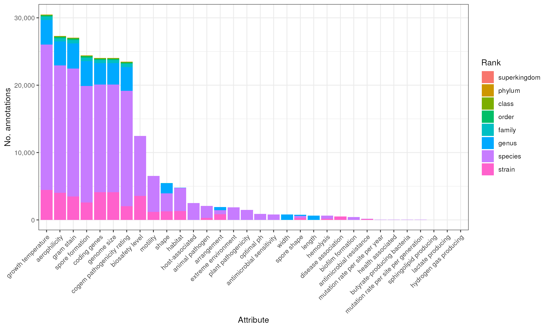
Total number of annotations by type of Evidence
count_types <- bp |>
    map (~{
        .x |>
            mutate(
                Type = case_when(
                    Evidence %in% c("exp", "igc", "nas", "tas") ~ "Source",
                    Evidence == "asr" ~ "ASR",
                    Evidence == "tax" ~ "IBD"
                )
            ) |>
            count(Attribute, Type)
}) |>
    bind_rows()


keep_attrs <- split(count_types, count_types$Attribute) |>
    keep( ~ {
        types <- unique(.x$Type)
        "IBD" %in% types | "ASR" %in% types
    }) |>
    names()

p_count_types <- count_types |>
    filter(Attribute %in% keep_attrs) |>
    mutate(Attribute = factor(Attribute, levels = attr_order)) |>
    ggplot(aes(Attribute, n)) +
    geom_col(aes(fill = Type), position = "stack") +
    labs(
        x = "Attribute", y = "No. annotations"
    ) +
    scale_fill_discrete(name = "Annotation types") +
    scale_y_continuous(labels = scales::comma) +
    theme_bw() +
    theme(axis.text.x = element_text(angle = 45, hjust = 1))
p_count_types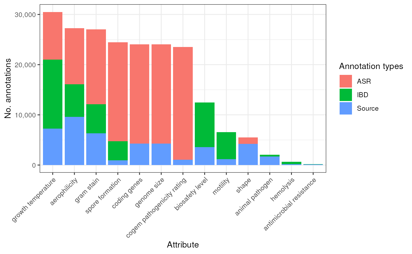
Figure: 10-fold cross-validation and counts per evidence type (species)
Create plot of MMC values for discrete attributes:
# val_fname <- "/home/samuelgamboa/Projects/taxPProValidation/validation_summary.tsv"
# val <- readr::read_tsv(val_fname, show_col_types = FALSE) |>
#     filter(rank == "all")
val <- bugphyzz:::.validationData() |>
filter(rank == "all") # Validation including taxa of mixed ranks as input (keyword is "all")
dis_phys_names <- val |>
    filter(!is.na(mcc_mean)) |>
    group_by(physiology) |>
    slice_max(order_by = mcc_mean, n = 1) |>
    arrange(-mcc_mean) |>
    pull(physiology)
pValDis <- val |> # plot Validation Discrete
    filter(!is.na(mcc_mean))  |>
    mutate(ltp_bp = ifelse(is.na(ltp_bp), ltp_bp_phys, ltp_bp)) |>
    mutate(physiology = factor(physiology, levels = dis_phys_names)) |>
    mutate(
        guide_col = ifelse(
            as.character(physiology) == attribute,
            as.character(physiology),
            paste0(as.character(physiology), "|", attribute)
        )
    ) |>
    arrange(physiology, mcc_mean) |>
    ggplot(aes(forcats::fct_inorder(guide_col), mcc_mean, group = attribute)) +
    geom_errorbar(
        aes(ymin = mcc_mean - mcc_sd, ymax = mcc_mean + mcc_sd),
        position = position_dodge(0.5),
        width = 0, linewidth = 0.3

    ) +
    geom_hline(
        yintercept = 0.7, linetype = "dotdash", linewidth = 0.2,
        color = "red"
    ) +
    geom_point(
        aes(size = ltp_bp),
        shape = 23, position = position_dodge(0.5), fill = "white"
        # size = 2
    ) +
    scale_size_continuous(name = "tips annotated") +
    scale_y_continuous(
        breaks = round(
            seq(
                min(val$mcc_mean - val$mcc_sd, na.rm = TRUE) - 0.1,
                max(val$mcc_mean + val$mcc_sd, na.rm = TRUE) + 0.1,
                0.2),
            1)
    ) +
    labs(
        y = "Matthews Correlation Coefficient",
        x = "Attribute|Attribute value"
    ) +
    theme_bw()  +
    theme(
        panel.grid.minor = element_blank()

    ) +
    coord_flip()
Create plot of R-squared values for continuous attributes:
num <- val |>
    filter(!is.na(r2_mean))
num_phys_names <- num |>
    group_by(physiology) |>
    slice_max(order_by = r2_mean, n = 1) |>
    arrange(-r2_mean) |>
    pull(physiology)
pValNum <- val |>  # plot Validation Numeric attributes
    filter(!is.na(r2_mean))  |>
    mutate(ltp_bp = ifelse(is.na(ltp_bp), ltp_bp_phys, ltp_bp)) |>
    ggplot(aes(reorder(physiology, -r2_mean), r2_mean, group = attribute)) +
    geom_errorbar(
        aes(ymin = r2_mean - r2_sd, ymax = r2_mean + r2_sd),
        position = position_dodge(0.5),
        width = 0, linewidth = 0.3

    ) +
    geom_hline(
        yintercept = 0.5, linetype = "dotdash", linewidth = 0.2,
        color = "red"
    ) +
    geom_point(
        aes(size = ltp_bp),
        shape = 23, position = position_dodge(0.5), fill = "white"
        # size = 2
    ) +
    scale_size_continuous(name = "tips annotated") +
    scale_y_continuous(
        breaks = round(seq(min(val$r2_mean - val$r2_sd, na.rm = TRUE) - 0.1, max(val$r2_mean + val$r2_sd, na.rm = TRUE) + 0.1, 0.2), 1)

    ) +
    labs(
        y = "R-squared",
        x = "Attribute"
    ) +
    theme_bw()  +
    theme(
        panel.grid.minor = element_blank()

    ) +
    coord_flip()
Crete plot of counts of annotations at the species level. Stack colors/columns with colors according to Evidence type of the annotations: ASR, IBD, Source. Only include attributes that were expanded with IBD or ASR.
counts_type_sp <- bp |>
    map(~ {
        .x |>
            filter(Rank == "species") |>
            mutate(
                Evidence = case_when(
                    Evidence == "tax" ~ "IBD",
                    Evidence == "asr" ~ "ASR",
                    Evidence %in% c("exp", "igc", "tas", "nas") ~ "Source",
                    TRUE ~ Evidence
                )
            ) |>
            count(Attribute, Evidence) |>
            mutate(total = sum(n))
    }) |>
    bind_rows()
p_counts_sp <- counts_type_sp |>
    filter(Attribute %in% keep_attrs) |>
    mutate(Evidence = factor(Evidence, levels = c("ASR", "IBD", "Source"))) |>
    ggplot(aes(reorder(Attribute, total), n)) +
    geom_col(aes(fill = Evidence), position = "stack") +
    labs(
        y = "No. annotations (species)", x = "Attribute"
    ) +
    scale_fill_manual(
        values = c("#56B4E9", "#D55E00", "#0072B2"),
        name = "Annotation type"
    ) +
    scale_y_continuous(labels = scales::comma) +
    theme_bw() +
    coord_flip()
Merge the plots from the validation results and the counts of annotations
myPlot2 <- plot_grid(
    pValNum, p_counts_sp, ncol = 1,
    labels = c("b)", "c)"),
    rel_heights = c(0.2, 0.8), align = "v"
)
myPlot1 <- plot_grid(
    pValDis, myPlot2,
    labels = c("a)"),
    rel_widths = c(0.55, 0.45), axis = "b"

)
myPlot1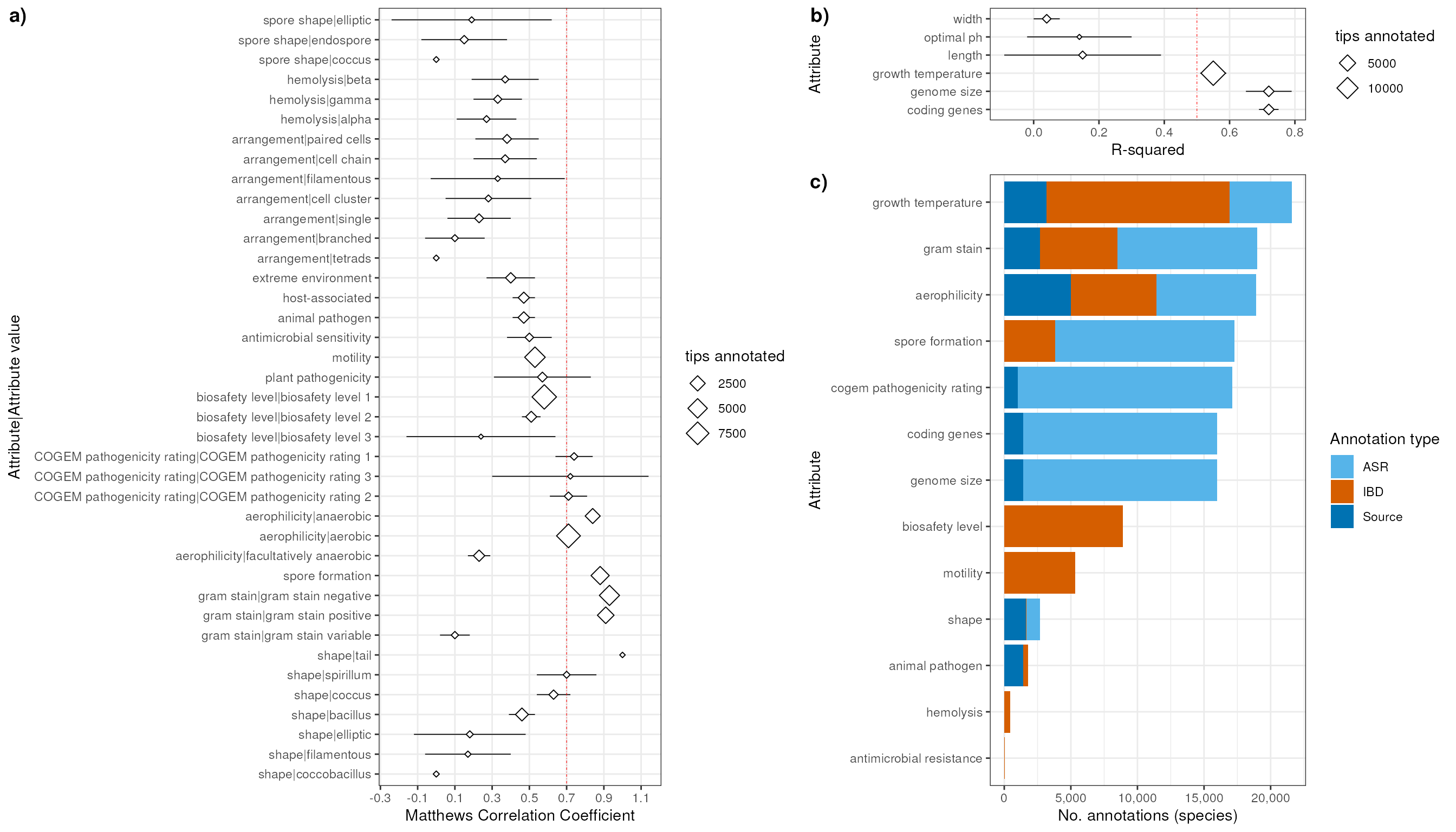
myDataTable(counts_type_sp)Supplementary Figure: Counts of annotations for genus, spescies, and strain and number of annotations per taxon
Number of annotations at the genus, species, and strain level:
counts_type_2 <- bp |>
    map(~ {
        .x |>
            filter(Rank %in% c("genus", "species", "strain")) |>
            mutate(
                Evidence = case_when(
                    Evidence == "tax" ~ "IBD",
                    Evidence == "asr" ~ "ASR",
                    Evidence %in% c("exp", "igc", "tas", "nas") ~ "Source",
                    TRUE ~ Evidence
                )
            ) |>
            count(Attribute, Rank, Evidence) |>
            mutate(total = sum(n))
    }) |>
    bind_rows()
p_counts_2 <- counts_type_2 |>
    filter(Attribute %in% keep_attrs) |>
    mutate(Evidence = factor(Evidence, levels = c("ASR", "IBD", "Source"))) |>
    ggplot(aes(reorder(Attribute, total), n)) +
    geom_col(aes(fill = Evidence), position = "stack") +
    labs(
        y = "No. annotations", x = "Attribute"
    ) +
    scale_fill_manual(
        values = c("#56B4E9", "#D55E00", "#0072B2"),
        name = "Annotation type"
    ) +
    scale_y_continuous(labels = scales::comma) +
    theme_bw() +
    facet_wrap(~Rank, nrow = 1, scales = "free_x") +
    theme(
        axis.text.x = element_text(angle = 45, hjust = 1)
    ) +
    coord_flip()
Frequency of number of annotations per single taxon:
n_annot_tax <- bp |>
   map(~ {
       attr_type <- unique(.x$Attribute_type)
       .x |>
           filter(Rank %in% c("strain", "species", "genus")) |>
           select(Attribute, NCBI_ID, Rank)
   }) |>
    bind_rows() |>
    count(NCBI_ID, Rank)
p_n_annot_tax <- n_annot_tax |>
    ggplot() +
    geom_histogram(aes(x = n), binwidth = 1) +
    labs(
        x = "Annotations per\ntaxon",
        y = "Frequency"
    ) +
    facet_wrap(~Rank, ncol = 1) +
    theme_bw()
Merge plots above for supplementary figure:
suppN <- plot_grid(
    p_counts_2, p_n_annot_tax,
    labels = c("a)", "b)"),
    rel_widths = c(0.8, 0.20),
    nrow = 1
)
suppN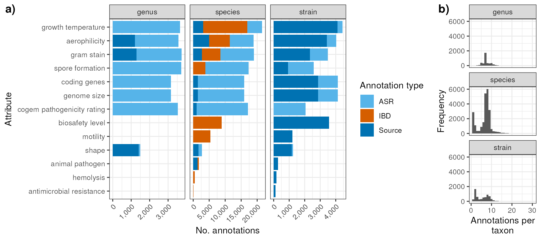
Figure: Heatmap Sources x Attribute x Rank
mySources <- bp |>
    map(~ {
        .x |>
            select(Attribute_source, Confidence_in_curation, Evidence) |>
            drop_na() |>
            rename(Confidence = Confidence_in_curation)
    }) |>
    bind_rows() |>
    distinct() |>
    mutate(
        Confidence_color = case_when(
            Confidence == "high" ~  "red",
            Confidence == "medium" ~ "orange",
            Confidence == "low" ~ "yellow"
        ),
        Evindence_color = case_when(
           Evidence == "exp" ~ "blue",
           Evidence == "igc" ~ "green",
           Evidence == "tas" ~ "brown4",
           Evidence == "nas" ~ "purple"
        ),
        Confidence = factor(Confidence, levels = c("high", "medium", "low")),
        Evidence = factor(Evidence, levels = c("exp", "igc", "tas", "nas"))
    )
source_attribute_rank <- bp |>
    map(~{
        .x |>
            filter(!is.na(Attribute_source)) |>
            count(Attribute, Attribute_source, Rank)
    }) |>
    bind_rows()

mat <- source_attribute_rank |>
    arrange(Attribute, Rank) |>
    unite(col = "Attribute|Rank", Attribute, Rank, sep = "|") |>
    pivot_wider(
        names_from = "Attribute_source", values_from = "n"
    ) |>
    tibble::column_to_rownames(var = "Attribute|Rank") |>
    as.data.frame() |>
    as.matrix()
mat[is.na(mat)] <- 0
mat[mat > 0] <- 1

color_fun <- circlize::colorRamp2(
  breaks = c(0, 1), colors = c('white', "gray20")
)
rankAnnotationsDF <- data.frame(
    Rank = sub("^(.*\\|)(\\w+)$", "\\2", rownames(mat))
)
rank_colors =list(
    Rank = c("genus" = "orange","species" = "#009E73", "strain" = "#CC79A7")
)
row_ha <- rowAnnotation(
    df = rankAnnotationsDF, col = rank_colors, width = unit(5, "cm")
)

mySources <- mySources[match(colnames(mat), mySources$Attribute_source),]

myColColors <- list(
    Confidence = c(high = "red", medium = "orange", low = "yellow"),
    Evidence = c(exp = "blue", igc = "green", tas = "pink3", nas = "purple")
)
column_ha <- columnAnnotation(
    df = mySources[, c("Confidence", "Evidence")],
    col = myColColors,
    height = unit(5, "cm")
)

splits_attrs <- sub("^(.*)\\|\\w+$", "\\1", rownames(mat))
hp <- Heatmap(
    matrix = mat,
    cluster_rows = FALSE,
    cluster_columns = FALSE,
    show_row_names = FALSE,
    show_heatmap_legend = TRUE,
    col = color_fun(c(0, 1)),
    name = "Annotation presence",
    left_annotation = row_ha,
    bottom_annotation = column_ha,
    row_split = splits_attrs,
    row_title_rot = 0,
    heatmap_legend_param = list(
        color_bar = "discrete",
        border = "black"
    ),
    border = TRUE,
    rect_gp = gpar(col = "gray50", lwd = 1),
    column_names_max_height = unit(7, "cm")
)
hp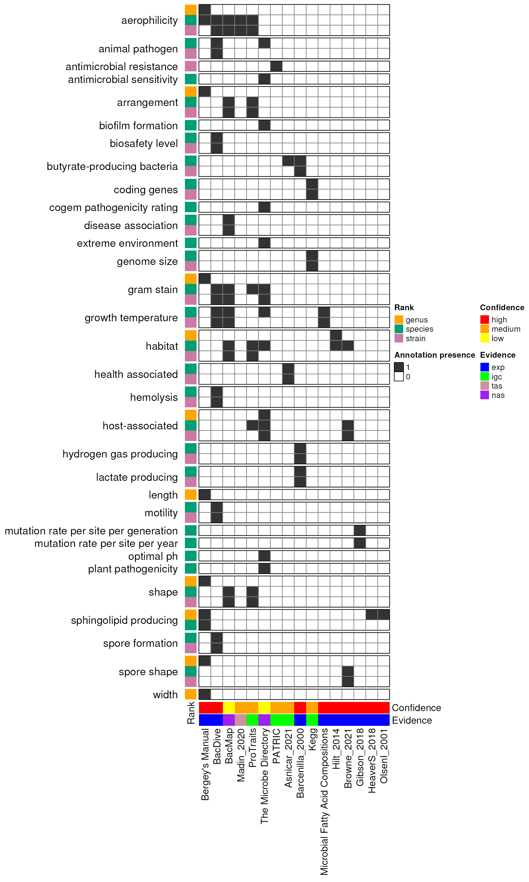
Table/Sup Table: Sources
sources_fname <- system.file(
    "extdata", "attribute_sources.tsv", package = "bugphyzz", mustWork = TRUE
)
sources <- read.table(
    file = sources_fname,
    header = TRUE, sep = "\t",  quote = ""
) |>
    rename(
        `Source (short)` = Attribute_source,
        `Confidence in curation` = Confidence_in_curation,
        `Source (long)` = full_source
    )
myDataTable(sources, page_len = nrow(sources))
Session information
sessioninfo::session_info()
#> ─ Session info ───────────────────────────────────────────────────────────────
#>  setting  value
#>  version  R version 4.4.1 (2024-06-14)
#>  os       Ubuntu 22.04.4 LTS
#>  system   x86_64, linux-gnu
#>  ui       X11
#>  language en
#>  collate  en_US.UTF-8
#>  ctype    en_US.UTF-8
#>  tz       Etc/UTC
#>  date     2024-06-28
#>  pandoc   3.2 @ /usr/bin/ (via rmarkdown)
#>
#> ─ Packages ───────────────────────────────────────────────────────────────────
#>  package              * version date (UTC) lib source
#>  abind                  1.4-5   2016-07-21 [1] RSPM (R 4.4.0)
#>  aplot                  0.2.3   2024-06-17 [1] RSPM (R 4.4.0)
#>  backports              1.5.0   2024-05-23 [1] RSPM (R 4.4.0)
#>  Biobase              * 2.64.0  2024-04-30 [1] Bioconductor 3.19 (R 4.4.1)
#>  BiocFileCache          2.12.0  2024-04-30 [1] Bioconductor 3.19 (R 4.4.1)
#>  BiocGenerics         * 0.50.0  2024-04-30 [1] Bioconductor 3.19 (R 4.4.1)
#>  bit                    4.0.5   2022-11-15 [1] RSPM (R 4.4.0)
#>  bit64                  4.0.5   2020-08-30 [1] RSPM (R 4.4.0)
#>  blob                   1.2.4   2023-03-17 [1] RSPM (R 4.4.0)
#>  broom                  1.0.6   2024-05-17 [1] RSPM (R 4.4.0)
#>  bslib                  0.7.0   2024-03-29 [1] RSPM (R 4.4.0)
#>  bugphyzz             * 0.99.3  2024-06-28 [1] Github (waldronlab/bugphyzz@8fc1c6d)
#>  bugphyzzAnalyses     * 0.1.19  2024-06-28 [1] local
#>  cachem                 1.1.0   2024-05-16 [1] RSPM (R 4.4.0)
#>  Cairo                  1.6-2   2023-11-28 [1] RSPM (R 4.4.0)
#>  car                    3.1-2   2023-03-30 [1] RSPM (R 4.4.0)
#>  carData                3.0-5   2022-01-06 [1] RSPM (R 4.4.0)
#>  circlize               0.4.16  2024-02-20 [1] RSPM (R 4.4.0)
#>  cli                    3.6.3   2024-06-21 [1] RSPM (R 4.4.0)
#>  clue                   0.3-65  2023-09-23 [1] RSPM (R 4.4.0)
#>  cluster                2.1.6   2023-12-01 [2] CRAN (R 4.4.1)
#>  codetools              0.2-20  2024-03-31 [2] CRAN (R 4.4.1)
#>  colorspace             2.1-0   2023-01-23 [1] RSPM (R 4.4.0)
#>  ComplexHeatmap       * 2.20.0  2024-04-30 [1] Bioconductor 3.19 (R 4.4.1)
#>  cowplot              * 1.1.3   2024-01-22 [1] RSPM (R 4.4.0)
#>  crayon                 1.5.3   2024-06-20 [1] RSPM (R 4.4.0)
#>  crosstalk              1.2.1   2023-11-23 [1] RSPM (R 4.4.0)
#>  curl                   5.2.1   2024-03-01 [1] RSPM (R 4.4.0)
#>  DBI                    1.2.3   2024-06-02 [1] RSPM (R 4.4.0)
#>  dbplyr                 2.5.0   2024-03-19 [1] RSPM (R 4.4.0)
#>  DelayedArray           0.30.1  2024-05-07 [1] Bioconductor 3.19 (R 4.4.1)
#>  desc                   1.4.3   2023-12-10 [1] RSPM (R 4.4.0)
#>  digest                 0.6.36  2024-06-23 [1] RSPM (R 4.4.0)
#>  doParallel             1.0.17  2022-02-07 [1] RSPM (R 4.4.0)
#>  dplyr                * 1.1.4   2023-11-17 [1] RSPM (R 4.4.0)
#>  DT                     0.33    2024-04-04 [1] RSPM (R 4.4.0)
#>  evaluate               0.24.0  2024-06-10 [1] RSPM (R 4.4.0)
#>  fansi                  1.0.6   2023-12-08 [1] RSPM (R 4.4.0)
#>  farver                 2.1.2   2024-05-13 [1] RSPM (R 4.4.0)
#>  fastmap                1.2.0   2024-05-15 [1] RSPM (R 4.4.0)
#>  filelock               1.0.3   2023-12-11 [1] RSPM (R 4.4.0)
#>  forcats              * 1.0.0   2023-01-29 [1] RSPM (R 4.4.0)
#>  foreach                1.5.2   2022-02-02 [1] RSPM (R 4.4.0)
#>  fs                     1.6.4   2024-04-25 [1] RSPM (R 4.4.0)
#>  generics               0.1.3   2022-07-05 [1] RSPM (R 4.4.0)
#>  GenomeInfoDb         * 1.40.1  2024-05-24 [1] Bioconductor 3.19 (R 4.4.1)
#>  GenomeInfoDbData       1.2.12  2024-06-25 [1] Bioconductor
#>  GenomicRanges        * 1.56.1  2024-06-12 [1] Bioconductor 3.19 (R 4.4.1)
#>  GetoptLong             1.0.5   2020-12-15 [1] RSPM (R 4.4.0)
#>  ggbreak              * 0.1.2   2023-06-26 [1] RSPM (R 4.4.0)
#>  ggfun                  0.1.5   2024-05-28 [1] RSPM (R 4.4.0)
#>  ggplot2              * 3.5.1   2024-04-23 [1] RSPM (R 4.4.0)
#>  ggplotify              0.1.2   2023-08-09 [1] RSPM (R 4.4.0)
#>  ggpubr               * 0.6.0   2023-02-10 [1] RSPM (R 4.4.0)
#>  ggsignif               0.6.4   2022-10-13 [1] RSPM (R 4.4.0)
#>  GlobalOptions          0.1.2   2020-06-10 [1] RSPM (R 4.4.0)
#>  glue                   1.7.0   2024-01-09 [1] RSPM (R 4.4.0)
#>  gridGraphics           0.5-1   2020-12-13 [1] RSPM (R 4.4.0)
#>  gtable                 0.3.5   2024-04-22 [1] RSPM (R 4.4.0)
#>  highr                  0.11    2024-05-26 [1] RSPM (R 4.4.0)
#>  htmltools              0.5.8.1 2024-04-04 [1] RSPM (R 4.4.0)
#>  htmlwidgets            1.6.4   2023-12-06 [1] RSPM (R 4.4.0)
#>  httr                   1.4.7   2023-08-15 [1] RSPM (R 4.4.0)
#>  httr2                  1.0.1   2024-04-01 [1] RSPM (R 4.4.0)
#>  IRanges              * 2.38.0  2024-04-30 [1] Bioconductor 3.19 (R 4.4.1)
#>  iterators              1.0.14  2022-02-05 [1] RSPM (R 4.4.0)
#>  jquerylib              0.1.4   2021-04-26 [1] RSPM (R 4.4.0)
#>  jsonlite               1.8.8   2023-12-04 [1] RSPM (R 4.4.0)
#>  knitr                  1.47    2024-05-29 [1] RSPM (R 4.4.0)
#>  labeling               0.4.3   2023-08-29 [1] RSPM (R 4.4.0)
#>  lattice                0.22-6  2024-03-20 [2] CRAN (R 4.4.1)
#>  lifecycle              1.0.4   2023-11-07 [1] RSPM (R 4.4.0)
#>  magick                 2.8.3   2024-02-18 [1] RSPM (R 4.4.0)
#>  magrittr               2.0.3   2022-03-30 [1] RSPM (R 4.4.0)
#>  Matrix                 1.7-0   2024-04-26 [2] CRAN (R 4.4.1)
#>  MatrixGenerics       * 1.16.0  2024-04-30 [1] Bioconductor 3.19 (R 4.4.1)
#>  matrixStats          * 1.3.0   2024-04-11 [1] RSPM (R 4.4.0)
#>  memoise                2.0.1   2021-11-26 [1] RSPM (R 4.4.0)
#>  munsell                0.5.1   2024-04-01 [1] RSPM (R 4.4.0)
#>  patchwork            * 1.2.0   2024-01-08 [1] RSPM (R 4.4.0)
#>  pillar                 1.9.0   2023-03-22 [1] RSPM (R 4.4.0)
#>  pkgconfig              2.0.3   2019-09-22 [1] RSPM (R 4.4.0)
#>  pkgdown                2.0.9   2024-04-18 [1] RSPM (R 4.4.0)
#>  png                    0.1-8   2022-11-29 [1] RSPM (R 4.4.0)
#>  purrr                * 1.0.2   2023-08-10 [1] RSPM (R 4.4.0)
#>  R6                     2.5.1   2021-08-19 [1] RSPM (R 4.4.0)
#>  ragg                   1.3.2   2024-05-15 [1] RSPM (R 4.4.0)
#>  rappdirs               0.3.3   2021-01-31 [1] RSPM (R 4.4.0)
#>  RColorBrewer           1.1-3   2022-04-03 [1] RSPM (R 4.4.0)
#>  Rcpp                   1.0.12  2024-01-09 [1] RSPM (R 4.4.0)
#>  rjson                  0.2.21  2022-01-09 [1] RSPM (R 4.4.0)
#>  rlang                  1.1.4   2024-06-04 [1] RSPM (R 4.4.0)
#>  rmarkdown              2.27    2024-05-17 [1] RSPM (R 4.4.0)
#>  RSQLite                2.3.7   2024-05-27 [1] RSPM (R 4.4.0)
#>  rstatix                0.7.2   2023-02-01 [1] RSPM (R 4.4.0)
#>  S4Arrays               1.4.1   2024-05-20 [1] Bioconductor 3.19 (R 4.4.1)
#>  S4Vectors            * 0.42.0  2024-04-30 [1] Bioconductor 3.19 (R 4.4.1)
#>  sass                   0.4.9   2024-03-15 [1] RSPM (R 4.4.0)
#>  scales                 1.3.0   2023-11-28 [1] RSPM (R 4.4.0)
#>  sessioninfo            1.2.2   2021-12-06 [1] RSPM (R 4.4.0)
#>  shape                  1.4.6.1 2024-02-23 [1] RSPM (R 4.4.0)
#>  SparseArray            1.4.8   2024-05-24 [1] Bioconductor 3.19 (R 4.4.1)
#>  stringi                1.8.4   2024-05-06 [1] RSPM (R 4.4.0)
#>  stringr                1.5.1   2023-11-14 [1] RSPM (R 4.4.0)
#>  SummarizedExperiment * 1.34.0  2024-05-01 [1] Bioconductor 3.19 (R 4.4.1)
#>  systemfonts            1.1.0   2024-05-15 [1] RSPM (R 4.4.0)
#>  taxPPro              * 1.0.0   2024-06-28 [1] Github (waldronlab/taxPPro@b0460fe)
#>  textshaping            0.4.0   2024-05-24 [1] RSPM (R 4.4.0)
#>  tibble               * 3.2.1   2023-03-20 [1] RSPM (R 4.4.0)
#>  tidyr                * 1.3.1   2024-01-24 [1] RSPM (R 4.4.0)
#>  tidyselect             1.2.1   2024-03-11 [1] RSPM (R 4.4.0)
#>  UCSC.utils             1.0.0   2024-04-30 [1] Bioconductor 3.19 (R 4.4.1)
#>  utf8                   1.2.4   2023-10-22 [1] RSPM (R 4.4.0)
#>  vctrs                  0.6.5   2023-12-01 [1] RSPM (R 4.4.0)
#>  withr                  3.0.0   2024-01-16 [1] RSPM (R 4.4.0)
#>  xfun                   0.45    2024-06-16 [1] RSPM (R 4.4.0)
#>  XVector                0.44.0  2024-04-30 [1] Bioconductor 3.19 (R 4.4.1)
#>  yaml                   2.3.8   2023-12-11 [1] RSPM (R 4.4.0)
#>  yulab.utils            0.1.4   2024-01-28 [1] RSPM (R 4.4.0)
#>  zlibbioc               1.50.0  2024-04-30 [1] Bioconductor 3.19 (R 4.4.1)
#>
#>  [1] /usr/local/lib/R/site-library
#>  [2] /usr/local/lib/R/library
#>
#> ──────────────────────────────────────────────────────────────────────────────