bugphyzz
A harmonized data resource and software for enrichment analysis of microbial physiologies
Samuel Gamboa
Samuel.Gamboa.Tuz@gmail.comLevi Waldron
levi.waldron@sph.cuny.edu Source:vignettes/bugphyzz.Rmd
bugphyzz.RmdAbstract
The bugphyzz package simplifies the import of
harmonized microbial annotations into R from diverse sources.
These annotations, including extended taxa via ancestral state
reconstruction, are organized into tidy data.frame
objects, facilitating the creation of microbial signatures. These
signatures can be used for enrichment analysis of microbiome omic
data, akin to gene set enrichment analysis using tools like EnrichmentBrowser
and bugsigdbr,
which are also available on Bioconductor. Annotaions are imported
from Zenodo.
Introduction
The bugphyzz package offers a convenient way to import a collection
of harmonized microbial annotations from various sources into R. These
annotations are available on Zenodo. In
addition to being harmonized, some annotations have been extended to
other taxa based on the phylogeny from ‘The All-Species Living Tree
Project’ using ancestral state reconstruction (ASR) methods. The
annotations are provided in tabular format and organized into distinct
tidy data.frame objects (for details, see the “Data schema”
section below).
Once imported, these data.frame objects can be used to
create microbial signatures, which are lists of taxa with shared
characteristics. We anticipate these signatures being utilized for
enrichment analysis of microbiome omic data by implementing workflows
similar to those used in gene set enrichment analysis; for example,
using the EnrichmentBrowser
package (a detailed example is provided in a section below).
A similar package in Bioconductor is the bugsigdbr package, which imports literature-published microbial signatures from the BugSigDB database and has been used for bug set enrichment analysis (BSEA). Moreover, the writeGMT function from the bugsigdbr package can export bugphyzz signatures as GMT text files.
Data schema
Annotations in bugphyzz represent the link between a taxon (Bacteria/Archaea) and an attribute, as outlined in the data schema provided below.
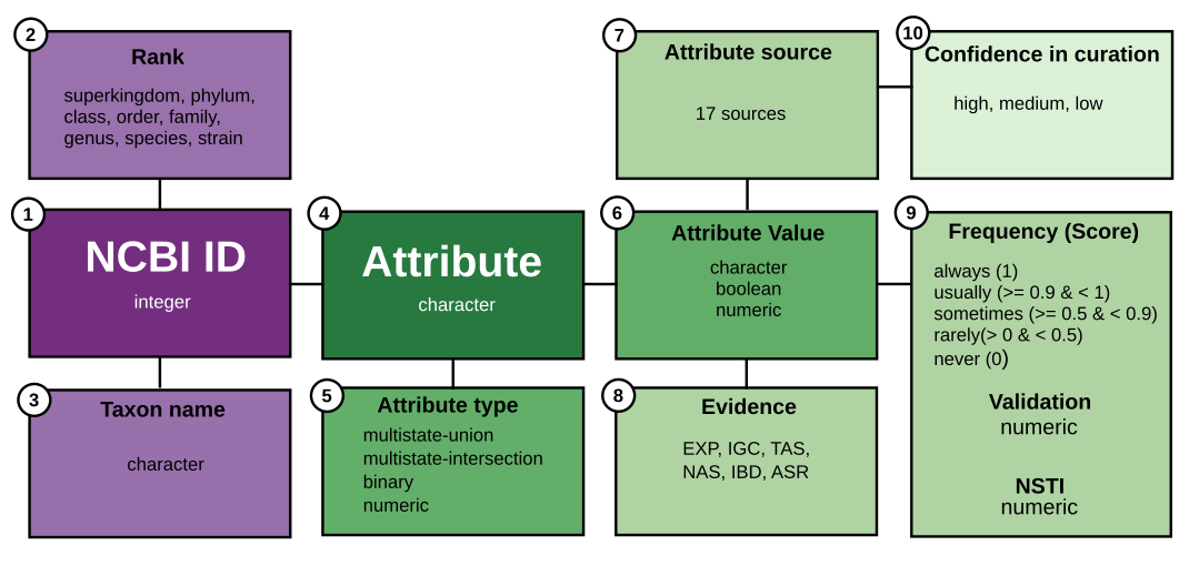
Taxon-related
Taxonomic data in bugphyzz is standardized according to the NCBI taxonomy:
- NCBI ID: An integer representing the NCBI taxonomy ID (taxid) associated with a taxon.
- Rank: A character string indicating the taxonomy rank, including superkingdom, kingdom, phylum, class, order, family, genus, species, or strain.
- Taxon name: A character string denoting the scientific name of the taxon.
Attribute-related
Attribute data is harmonized using ontology terms. Details of attributes, ontology terms, and ontology libraries can be found in the Attribute and sources article.
- Attribute: A character string describing the name of a trait that can be observed or measured.
-
Attribute type: A character string indicating the data
type:
- numeric: Attributes with numeric values (e.g., growth temperature: 25°C).
- binary: Attributes with boolean values (e.g., butyrate-producing: TRUE).
- multistate-intersection: A set of related binary attributes (e.g., habitat).
- multistate-union: Attributes with three or more values represented as character strings (e.g., aerophilicity: aerobic, anaerobic, or facultatively anaerobic).
- Attribute value: The possible values that an attribute could take, represented as character strings, booleans, or numbers.
Attribute value-related
Metadata associated with attribute values:
- Attribute source: The source of the information.
-
Evidence: The type of evidence supporting an annotation,
including:
- EXP: Experiment
- IGC: Inferred from genomic context
- TAS: Traceable author statement
- NAS: Non-traceable author statement
- IBD: Inferred from biological aspect of descendant
- ASR: Ancestral state reconstruction
-
Support values:
- Frequency and Score: Confidence that a given taxon exhibits a trait based on the curator’s knowledge or results of ASR or IBD.
- Validation: Score from the 10-fold cross-validation analysis. Matthews correlation coefficient (MCC) for discrete attributes and R-squared for numeric attributes. Default threshold value is 0.5 and above.
- NSTI: Nearest sequence taxon index from PICRUSt2 or the castor package. Relevant for numeric values only.
Attribute source-related
- Confidence in curation: A character string indicating the confidence value of a source based on three criteria: 1) presence of a source, 2) valid references, and 3) peer-reviewed curation. Valid options include high, medium, or low, corresponding to satisfaction of three, two, or one of these criteria.
Additional information
Description of sources and attributes: https://waldronlab.io/bugphyzz/articles/attributes.html
Description of ontology evidence codes: https://geneontology.org/docs/guide-go-evidence-codes/
Description of frequency keywords and scores were based on: https://grammarist.com/grammar/adverbs-of-frequency/
IBD and ASR were performed with taxPPro: https://github.com/waldronlab/taxPPro
Analysis and Stats
This vignette serves as an introduction to the basic functionalities of bugphyzz. For a more in-depth analysis and detailed statistics utilizing bugphyzz annotations, please visit: https://github.com/waldronlab/bugphyzzAnalyses
Installation
if (!require("BiocManager", quietly = TRUE))
    install.packages("BiocManager")

BiocManager::install("bugphyzz")
Import bugphyzz data
Load the bugphyzz package and additional packages for data manipulation:
bugphyzz data is imported using the importBugphyzz
function, resulting in a list of tidy data frames. Each data frame
corresponds to an attribute or a group of related attributes. This is
particularly evident in the case of the multistate-union type described
in the data schema above, where related attributes are grouped together
in a single data frame. Available attribute names can be inspected with
the names function:
bp <- importBugphyzz()
names(bp)
#>  [1] "animal pathogen"
#>  [2] "antimicrobial sensitivity"
#>  [3] "biofilm formation"
#>  [4] "butyrate-producing bacteria"
#>  [5] "extreme environment"
#>  [6] "health associated"
#>  [7] "host-associated"
#>  [8] "hydrogen gas producing"
#>  [9] "lactate producing"
#> [10] "motility"
#> [11] "plant pathogenicity"
#> [12] "sphingolipid producing"
#> [13] "spore formation"
#> [14] "aerophilicity"
#> [15] "antimicrobial resistance"
#> [16] "arrangement"
#> [17] "biosafety level"
#> [18] "cogem pathogenicity rating"
#> [19] "disease association"
#> [20] "gram stain"
#> [21] "habitat"
#> [22] "hemolysis"
#> [23] "shape"
#> [24] "spore shape"
#> [25] "coding genes"
#> [26] "genome size"
#> [27] "growth temperature"
#> [28] "length"
#> [29] "mutation rate per site per generation"
#> [30] "mutation rate per site per year"
#> [31] "optimal ph"
#> [32] "width"
Let’s take a glimpse at one of the data frames:
glimpse(bp$aerophilicity, width = 50)
#> Rows: 17,966
#> Columns: 12
#> $ NCBI_ID                <int> 117743, 118001, 1…
#> $ Taxon_name             <chr> "Flavobacteriia",…
#> $ Rank                   <chr> "class", "class",…
#> $ Attribute              <chr> "aerophilicity", …
#> $ Attribute_value        <chr> "anaerobic", "ana…
#> $ Evidence               <chr> "asr", "asr", "as…
#> $ Frequency              <chr> "sometimes", "usu…
#> $ Score                  <dbl> 0.6911516, 0.9992…
#> $ Attribute_source       <chr> NA, NA, NA, NA, N…
#> $ Confidence_in_curation <chr> NA, NA, NA, NA, N…
#> $ Attribute_type         <chr> "multistate-inter…
#> $ Validation             <dbl> 0.84, 0.84, 0.84,…
Compare the column names with the data schema described above.
Create microbial signatures
bugphyzz’s primary function is to facilitate the creation of
microbial signatures, which are essentially lists of microbes sharing
specific taxonomy ranks and attribute values. Once the data frames
containing attribute information are imported, the
makeSignatures function can be employed to generate these
signatures. makeSignatures offers various filtering
options, including evidence, frequency, and minimum and maximum values
for numeric attributes. For more precise filtering requirements, users
can leverage standard data manipulation functions on the relevant data
frame, such as dplyr::filter.
Examples:
- Create signatures of taxon names at the genus level for the aerophilicity attribute (discrete):
aer_sigs_g <- makeSignatures(
    dat = bp[["aerophilicity"]], taxIdType = "Taxon_name", taxLevel = "genus"
)
map(aer_sigs_g, head)
#> $`bugphyz:aerophilicity|aerobic`
#> [1] "Cellvibrio"     "Acidipila"      "Hydrotalea"     "Saprospira"
#> [5] "Nitrosarchaeum" "Halopelagius"
#>
#> $`bugphyz:aerophilicity|anaerobic`
#> [1] "Microaerobacter"      "Desulfitispora"       "Desulfurispira"
#> [4] "Pseudoflavonifractor" "Chromatium"           "Ectothiorhodospira"
#>
#> $`bugphyz:aerophilicity|facultatively anaerobic`
#> [1] "Capnocytophaga" "Kistimonas"     "Trueperella"    "Telmatobacter"
#> [5] "Alishewanella" "Muricauda"- Create signatures of taxon names at the species level for the growth temperature attribute (numeric):
gt_sigs_sp <- makeSignatures(
    dat = bp[["growth temperature"]], taxIdType = "Taxon_name",
    taxLevel = 'species'
)
map(gt_sigs_sp, head)
#> $`bugphyzz:growth temperature|hyperthermophile| > 60 & <= 121`
#> [1] "Metallosphaera cuprina"      "Pyrococcus yayanosii"
#> [3] "Methanothermobacter crinale" "Acidilobus aceticus"
#> [5] "Thermanaerovibrio velox"     "Thermoanaerobacter italicus"
#>
#> $`bugphyzz:growth temperature|mesophile| > 25 & <= 45`
#> [1] "Ancylobacter aquaticus"          "Leptospira alexanderi"
#> [3] "Halosaccharopolyspora lacisalsi" "Garritya polymorpha"
#> [5] "Sporobacterium olearium"         "Borreliella lusitaniae"
#>
#> $`bugphyzz:growth temperature|psychrophile| > -10.01 & <= 25`
#> [1] "Cryobacterium roopkundense"  "Hugenholtzia roseola"
#> [3] "Halopseudomonas formosensis" "Occallatibacter riparius"
#> [5] "Occallatibacter savannae"    "Pectinatus sottacetonis"
#>
#> $`bugphyzz:growth temperature|thermophile| > 45 & <= 60`
#> [1] "Alicyclobacillus cellulosilyticus" "Defluviitoga tunisiensis"
#> [3] "Fervidobacterium thailandense"     "Polycladomyces subterraneus"
#> [5] "Desulfofalx alkaliphila" "Marinitoga camini"- Create signatures with a custom threshold for the growth temperature attribute (numeric):
gt_sigs_mix <- makeSignatures(
    dat = bp[["growth temperature"]], taxIdType = "Taxon_name",
    taxLevel = "mixed", min = 0, max = 25
)
map(gt_sigs_mix, head)
#> $`bugphyzz:growth temperature| >=0 & <=25`
#> [1] "Cryobacterium roopkundense"  "Hugenholtzia roseola"
#> [3] "Halopseudomonas formosensis" "Occallatibacter riparius"
#> [5] "Occallatibacter savannae" "Pectinatus sottacetonis"- Create signatures for the animal pathogen attribute (boolean):
ap_sigs_mix <- makeSignatures(
    dat = bp[["animal pathogen"]], taxIdType = "NCBI_ID",
    taxLevel = "mixed", evidence = c("exp", "igc", "nas", "tas")
)
map(ap_sigs_mix, head)
#> $`bugphyz:animal pathogen|FALSE`
#> [1]  100225 1003110    1006    1008 1008460  101192
#>
#> $`bugphyz:animal pathogen|TRUE`
#> [1] 100053 100901 1015 1017 1018 1019- Create signatures for all of the bugphyzz data frames:
sigs <- map(bp, makeSignatures) |>
    list_flatten(name_spec = "{inner}")
length(sigs)
#> [1] 123
head(map(sigs, head))
#> $`bugphyz:animal pathogen|FALSE`
#> [1]  100225 1003110    1006    1008 1008460  101192
#>
#> $`bugphyz:animal pathogen|TRUE`
#> [1]  100053 1004150 1004159 1004165 1004166  100469
#>
#> $`bugphyz:antimicrobial sensitivity|FALSE`
#> [1]  100225    1008 1008460  101192  101385  101534
#>
#> $`bugphyz:antimicrobial sensitivity|TRUE`
#> [1] 1003110  100379  101564  101571    1031  103232
#>
#> $`bugphyz:biofilm formation|FALSE`
#> [1]    1006    1053  105841  105972 1079800  109790
#>
#> $`bugphyz:biofilm formation|TRUE`
#> [1]  100053    1018  102684  102862 1033739 1033846
Run a bug set enrichment analysis
Bugphyzz signatures are suitable for conducting bug set enrichment analysis using existing tools available in R. In this example, we will perform a set enrichment analysis using a dataset with a known biological ground truth.
The dataset originates from the Human Microbiome Project (2012) and compares subgingival and supragingival plaque. This data will be imported using the MicrobiomeBenchmarkData package. For the implementation of the enrichment analysis, we will utilize the Gene Set Enrichment Analysis (GSEA) method available in the EnrichmentBrowser package. The expected outcome is an enrichment of aerobic taxa in the supragingival plaque (positive enrichment score) and anaerobic taxa in the subgingival plaque (negative enrichment score).
Load necessary packages:
library(EnrichmentBrowser)
library(MicrobiomeBenchmarkData)
library(mia)
Import benchmark data:
dat_name <- 'HMP_2012_16S_gingival_V35'
tse <- MicrobiomeBenchmarkData::getBenchmarkData(dat_name, dryrun = FALSE)[[1]]
#> Finished HMP_2012_16S_gingival_V35.
tse_genus <- mia::splitByRanks(tse)$genus
min_n_samples <- round(ncol(tse_genus) * 0.2)
tse_subset <- tse_genus[rowSums(assay(tse_genus) >= 1) >= min_n_samples,]
tse_subset
#> class: TreeSummarizedExperiment
#> dim: 37 311
#> metadata(1): agglomerated_by_rank
#> assays(1): counts
#> rownames(37): Abiotrophia Actinobacillus ... Treponema Veillonella
#> rowData names(7): superkingdom phylum ... genus taxon_annotation
#> colnames(311): 700103497 700106940 ... 700111586 700109119
#> colData names(15): dataset subject_id ... sequencing_method
#>   variable_region_16s
#> reducedDimNames(0):
#> mainExpName: NULL
#> altExpNames(0):
#> rowLinks: a LinkDataFrame (37 rows)
#> rowTree: 1 phylo tree(s) (45364 leaves)
#> colLinks: NULL
#> colTree: NULL
Let’s use the edgeR method for differential abundance analysis and obtain sets of microbes. Subgingival plaque will be used as reference or “control”, so negative values will mean enrichment in the subgingival plaque and positive values will mean enrichment in the supragingival plaque.
Perform differential abundance (DA) analysis:
tse_subset$GROUP <- ifelse(
    tse_subset$body_subsite == 'subgingival_plaque', 0, 1
)
se <- EnrichmentBrowser::deAna(
    expr = tse_subset, de.method = 'edgeR', padj.method = 'fdr',
    filter.by.expr = FALSE,
)
It’s recommended to perform a normalization step of the counts before running GSEA. From the original GSEA user guide: “GSEA does not normalize RNA-seq data. RNA-seq data must be normalized for between-sample comparisons using an external normalization procedure (e.g. those in DESeq2 or Voom).”
In this example, we are treating the microbiome data as RNA-seq (see:
https://link.springer.com/article/10.1186/s13059-020-02104-1).
Let’s use the limma::voom function.
A glimpse to the assay stored in the SE:
assay(se)[1:5, 1:5] # counts
#>                 700103497 700106940 700097304 700099015 700097644
#> Abiotrophia             9        22        19         0         0
#> Actinobacillus          0         2         7         0         1
#> Actinomyces          1875      1012        12       499       248
#> Aggregatibacter      1084       157       215         0       144
#> Atopobium               1         0         1         0        18
From the ?limma::voom documentation, input should be “a
numeric matrix containing raw counts…”. Note that the assay in the
SummarizedExperiment will be replaced with normalized counts.
Perform normalization step:
dat <- data.frame(colData(se))
design <- stats::model.matrix(~ GROUP, data = dat)
assay(se) <- limma::voom(
    counts = assay(se), design = design, plot = FALSE
)$E
The output is a “numeric matrix of normalized expression values on
the log2 scale” as described in the ?lima::voom
documentation. This output is ready for GSEA.
assay(se)[1:5, 1:5] # normalized counts
#>                 700103497 700106940 700097304 700099015 700097644
#> Abiotrophia     10.038187 12.162796 12.294386  6.301074  4.935801
#> Actinobacillus   5.790260  8.992871 10.915875  6.301074  6.520764
#> Actinomyces     17.663319 17.654649 11.652840 16.265415 13.892903
#> Aggregatibacter 16.873074 14.970151 15.760528  6.301074 13.110727
#> Atopobium        7.375222  6.670943  8.593947  6.301074 10.145255
Perform GSEA and display the results:
gsea <- EnrichmentBrowser::sbea(
    method = 'gsea', se = se, gs = aer_sigs_g, perm = 1000,
    # Alpha is the FDR threshold (calculated above) to consider a feature as
    # significant.
    alpha = 0.1
)
gsea_tbl <- as.data.frame(gsea$res.tbl) |>
    mutate(
        GENE.SET = ifelse(PVAL < 0.05, paste0(GENE.SET, ' *'), GENE.SET),
        PVAL = round(PVAL, 3),
    ) |>
        dplyr::rename(BUG.SET = GENE.SET)
knitr::kable(gsea_tbl)| BUG.SET | ES | NES | PVAL |
|---|---|---|---|
| bugphyz:aerophilicity|aerobic * | 0.974 | 1.920 | 0.000 |
| bugphyz:aerophilicity|anaerobic * | -0.861 | -1.650 | 0.015 |
| bugphyz:aerophilicity|facultatively anaerobic | 0.317 | 0.709 | 0.810 |
Get signatures associated with a specific microbe
To retrieve all signature names associated with a specific taxon,
users can utilize the getTaxonSignatures function.
Let’s see an example using Escherichia coli (taxid: 562).
Get all signature names associated to E. coli:
getTaxonSignatures(tax = "Escherichia coli", bp = bp)
#> character(0)
Get all signature names associated to the E. coli taxid:
getTaxonSignatures(tax = "562", bp = bp)
#>  [1] "bugphyz:animal pathogen|FALSE"
#>  [2] "bugphyz:extreme environment|TRUE"
#>  [3] "bugphyz:health associated|FALSE"
#>  [4] "bugphyz:host-associated|TRUE"
#>  [5] "bugphyz:motility|FALSE"
#>  [6] "bugphyz:plant pathogenicity|FALSE"
#>  [7] "bugphyz:spore formation|FALSE"
#>  [8] "bugphyz:aerophilicity|aerobic"
#>  [9] "bugphyz:aerophilicity|facultatively anaerobic"
#> [10] "bugphyz:arrangement|paired cells"
#> [11] "bugphyz:biosafety level|biosafety level 1"
#> [12] "bugphyz:cogem pathogenicity rating|cogem pathogenicity rating 2"
#> [13] "bugphyz:gram stain|gram stain negative"
#> [14] "bugphyz:habitat|digestive system"
#> [15] "bugphyz:habitat|feces"
#> [16] "bugphyz:habitat|human microbiome"
#> [17] "bugphyz:shape|bacillus"
#> [18] "bugphyzz:growth temperature|mesophile| > 25 & <= 45"
#> [19] "bugphyzz:mutation rate per site per generation|slow| > 0.78 & <= 2.92"
#> [20] "bugphyzz:mutation rate per site per year|slow| > 0.08 & <= 7.5"
#> [21] "bugphyzz:optimal ph|neutral| > 6 & <= 8"
Session information
sessioninfo::session_info()
#> ─ Session info ───────────────────────────────────────────────────────────────
#>  setting  value
#>  version  R version 4.4.1 (2024-06-14)
#>  os       Ubuntu 22.04.5 LTS
#>  system   x86_64, linux-gnu
#>  ui       X11
#>  language en
#>  collate  en_US.UTF-8
#>  ctype    en_US.UTF-8
#>  tz       UTC
#>  date     2024-10-30
#>  pandoc   3.4 @ /usr/bin/ (via rmarkdown)
#>
#> ─ Packages ───────────────────────────────────────────────────────────────────
#>  package                  * version    date (UTC) lib source
#>  abind                      1.4-8      2024-09-12 [1] RSPM (R 4.4.0)
#>  annotate                   1.83.0     2024-05-01 [1] Bioconductor 3.20 (R 4.4.0)
#>  AnnotationDbi              1.67.0     2024-05-01 [1] Bioconductor 3.20 (R 4.4.0)
#>  ape                        5.8        2024-04-11 [1] RSPM (R 4.4.0)
#>  backports                  1.5.0      2024-05-23 [1] RSPM (R 4.4.0)
#>  base64enc                  0.1-3      2015-07-28 [2] RSPM (R 4.4.0)
#>  beachmat                   2.21.9     2024-10-27 [1] Bioconductor 3.20 (R 4.4.1)
#>  beeswarm                   0.4.0      2021-06-01 [1] RSPM (R 4.4.0)
#>  Biobase                  * 2.65.1     2024-10-21 [1] Bioconductor 3.20 (R 4.4.1)
#>  BiocFileCache              2.13.2     2024-10-21 [1] Bioconductor 3.20 (R 4.4.1)
#>  BiocGenerics             * 0.51.3     2024-10-21 [1] Bioconductor 3.20 (R 4.4.1)
#>  BiocManager                1.30.25    2024-08-28 [2] CRAN (R 4.4.1)
#>  BiocNeighbors              1.99.3     2024-10-21 [1] Bioconductor 3.20 (R 4.4.1)
#>  BiocParallel               1.39.0     2024-05-01 [1] Bioconductor 3.20 (R 4.4.0)
#>  BiocSingular               1.21.4     2024-10-21 [1] Bioconductor 3.20 (R 4.4.1)
#>  BiocStyle                * 2.33.1     2024-06-12 [1] Bioconductor 3.20 (R 4.4.0)
#>  Biostrings               * 2.73.2     2024-10-21 [1] Bioconductor 3.20 (R 4.4.1)
#>  bit                        4.5.0      2024-09-20 [1] RSPM (R 4.4.0)
#>  bit64                      4.5.2      2024-09-22 [1] RSPM (R 4.4.0)
#>  bitops                     1.0-9      2024-10-03 [1] RSPM (R 4.4.0)
#>  blob                       1.2.4      2023-03-17 [1] RSPM (R 4.4.0)
#>  bluster                    1.15.1     2024-10-21 [1] Bioconductor 3.20 (R 4.4.1)
#>  bookdown                   0.41       2024-10-16 [1] RSPM (R 4.4.0)
#>  boot                       1.3-31     2024-08-28 [2] RSPM (R 4.4.0)
#>  bslib                      0.8.0      2024-07-29 [2] RSPM (R 4.4.0)
#>  bugphyzz                 * 1.1.0      2024-10-30 [1] Bioconductor
#>  cachem                     1.1.0      2024-05-16 [2] RSPM (R 4.4.0)
#>  checkmate                  2.3.2      2024-07-29 [1] RSPM (R 4.4.0)
#>  cli                        3.6.3      2024-06-21 [2] RSPM (R 4.4.0)
#>  cluster                    2.1.6      2023-12-01 [3] CRAN (R 4.4.1)
#>  codetools                  0.2-20     2024-03-31 [3] CRAN (R 4.4.1)
#>  colorspace                 2.1-1      2024-07-26 [1] RSPM (R 4.4.0)
#>  crayon                     1.5.3      2024-06-20 [2] RSPM (R 4.4.0)
#>  curl                       5.2.3      2024-09-20 [2] RSPM (R 4.4.0)
#>  data.table                 1.16.2     2024-10-10 [1] RSPM (R 4.4.0)
#>  DBI                        1.2.3      2024-06-02 [1] RSPM (R 4.4.0)
#>  dbplyr                     2.5.0      2024-03-19 [1] RSPM (R 4.4.0)
#>  DECIPHER                   3.1.5      2024-10-21 [1] Bioconductor 3.20 (R 4.4.1)
#>  decontam                   1.25.0     2024-05-01 [1] Bioconductor 3.20 (R 4.4.0)
#>  DelayedArray               0.31.14    2024-10-21 [1] Bioconductor 3.20 (R 4.4.1)
#>  DelayedMatrixStats         1.27.3     2024-10-21 [1] Bioconductor 3.20 (R 4.4.1)
#>  desc                       1.4.3      2023-12-10 [2] RSPM (R 4.4.0)
#>  digest                     0.6.37     2024-08-19 [2] RSPM (R 4.4.0)
#>  DirichletMultinomial       1.47.2     2024-10-21 [1] Bioconductor 3.20 (R 4.4.1)
#>  dplyr                    * 1.1.4      2023-11-17 [1] RSPM (R 4.4.0)
#>  edgeR                      4.3.21     2024-10-25 [1] Bioconductor 3.20 (R 4.4.1)
#>  EnrichmentBrowser        * 2.35.1     2024-05-06 [1] Bioconductor 3.20 (R 4.4.0)
#>  evaluate                   1.0.1      2024-10-10 [2] RSPM (R 4.4.0)
#>  fansi                      1.0.6      2023-12-08 [2] RSPM (R 4.4.0)
#>  fastmap                    1.2.0      2024-05-15 [2] RSPM (R 4.4.0)
#>  filelock                   1.0.3      2023-12-11 [1] RSPM (R 4.4.0)
#>  foreign                    0.8-87     2024-06-26 [2] RSPM (R 4.4.0)
#>  Formula                    1.2-5      2023-02-24 [1] RSPM (R 4.4.0)
#>  fs                         1.6.4      2024-04-25 [2] RSPM (R 4.4.0)
#>  generics                   0.1.3      2022-07-05 [1] RSPM (R 4.4.0)
#>  GenomeInfoDb             * 1.41.2     2024-10-21 [1] Bioconductor 3.20 (R 4.4.1)
#>  GenomeInfoDbData           1.2.13     2024-10-25 [1] Bioconductor
#>  GenomicRanges            * 1.57.2     2024-10-21 [1] Bioconductor 3.20 (R 4.4.1)
#>  ggbeeswarm                 0.7.2      2023-04-29 [1] RSPM (R 4.4.0)
#>  ggplot2                    3.5.1      2024-04-23 [1] RSPM (R 4.4.0)
#>  ggrepel                    0.9.6      2024-09-07 [1] RSPM (R 4.4.0)
#>  glue                       1.8.0      2024-09-30 [2] RSPM (R 4.4.0)
#>  graph                    * 1.83.0     2024-05-01 [1] Bioconductor 3.20 (R 4.4.0)
#>  gridExtra                  2.3        2017-09-09 [1] RSPM (R 4.4.0)
#>  GSEABase                   1.67.1     2024-10-23 [1] Bioconductor 3.20 (R 4.4.1)
#>  gtable                     0.3.6      2024-10-25 [1] RSPM (R 4.4.0)
#>  Hmisc                      5.2-0      2024-10-28 [1] RSPM (R 4.4.0)
#>  htmlTable                  2.4.3      2024-07-21 [1] RSPM (R 4.4.0)
#>  htmltools                  0.5.8.1    2024-04-04 [2] RSPM (R 4.4.0)
#>  htmlwidgets                1.6.4      2023-12-06 [2] RSPM (R 4.4.0)
#>  httr                       1.4.7      2023-08-15 [1] RSPM (R 4.4.0)
#>  httr2                      1.0.5      2024-09-26 [2] RSPM (R 4.4.0)
#>  igraph                     2.1.1      2024-10-19 [1] RSPM (R 4.4.0)
#>  IRanges                  * 2.39.2     2024-10-21 [1] Bioconductor 3.20 (R 4.4.1)
#>  irlba                      2.3.5.1    2022-10-03 [1] RSPM (R 4.4.0)
#>  jquerylib                  0.1.4      2021-04-26 [2] RSPM (R 4.4.0)
#>  jsonlite                   1.8.9      2024-09-20 [2] RSPM (R 4.4.0)
#>  KEGGgraph                  1.65.0     2024-05-01 [1] Bioconductor 3.20 (R 4.4.0)
#>  KEGGREST                   1.45.1     2024-06-17 [1] Bioconductor 3.20 (R 4.4.0)
#>  knitr                      1.48       2024-07-07 [2] RSPM (R 4.4.0)
#>  lattice                    0.22-6     2024-03-20 [3] CRAN (R 4.4.1)
#>  lazyeval                   0.2.2      2019-03-15 [1] RSPM (R 4.4.0)
#>  lifecycle                  1.0.4      2023-11-07 [2] RSPM (R 4.4.0)
#>  limma                      3.61.12    2024-10-21 [1] Bioconductor 3.20 (R 4.4.1)
#>  lme4                       1.1-35.5   2024-07-03 [1] RSPM (R 4.4.0)
#>  locfit                     1.5-9.10   2024-06-24 [1] RSPM (R 4.4.0)
#>  lpSolve                    5.6.21     2024-09-12 [1] RSPM (R 4.4.0)
#>  magrittr                   2.0.3      2022-03-30 [2] RSPM (R 4.4.0)
#>  MASS                       7.3-61     2024-06-13 [2] RSPM (R 4.4.0)
#>  Matrix                     1.7-1      2024-10-18 [2] RSPM (R 4.4.0)
#>  MatrixGenerics           * 1.17.1     2024-10-23 [1] Bioconductor 3.20 (R 4.4.1)
#>  matrixStats              * 1.4.1      2024-09-08 [1] RSPM (R 4.4.0)
#>  mediation                  4.5.0      2019-10-08 [1] RSPM (R 4.4.0)
#>  memoise                    2.0.1      2021-11-26 [2] RSPM (R 4.4.0)
#>  mgcv                       1.9-1      2023-12-21 [3] CRAN (R 4.4.1)
#>  mia                      * 1.13.47    2024-10-22 [1] Bioconductor 3.20 (R 4.4.1)
#>  MicrobiomeBenchmarkData  * 1.7.1      2024-09-03 [1] Bioconductor 3.20 (R 4.4.1)
#>  minqa                      1.2.8      2024-08-17 [1] RSPM (R 4.4.0)
#>  MultiAssayExperiment     * 1.31.5     2024-10-21 [1] Bioconductor 3.20 (R 4.4.1)
#>  munsell                    0.5.1      2024-04-01 [1] RSPM (R 4.4.0)
#>  mvtnorm                    1.3-1      2024-09-03 [1] RSPM (R 4.4.0)
#>  nlme                       3.1-166    2024-08-14 [2] RSPM (R 4.4.0)
#>  nloptr                     2.1.1      2024-06-25 [1] RSPM (R 4.4.0)
#>  nnet                       7.3-19     2023-05-03 [3] CRAN (R 4.4.1)
#>  permute                    0.9-7      2022-01-27 [1] RSPM (R 4.4.0)
#>  pillar                     1.9.0      2023-03-22 [2] RSPM (R 4.4.0)
#>  pkgconfig                  2.0.3      2019-09-22 [2] RSPM (R 4.4.0)
#>  pkgdown                    2.1.1.9000 2024-10-30 [1] Github (r-lib/pkgdown@ffe60d5)
#>  plyr                       1.8.9      2023-10-02 [1] RSPM (R 4.4.0)
#>  png                        0.1-8      2022-11-29 [1] RSPM (R 4.4.0)
#>  purrr                    * 1.0.2      2023-08-10 [2] RSPM (R 4.4.0)
#>  R6                         2.5.1      2021-08-19 [2] RSPM (R 4.4.0)
#>  ragg                       1.3.3      2024-09-11 [2] RSPM (R 4.4.0)
#>  rappdirs                   0.3.3      2021-01-31 [2] RSPM (R 4.4.0)
#>  rbiom                      1.0.3      2021-11-05 [1] RSPM (R 4.4.0)
#>  Rcpp                       1.0.13     2024-07-17 [2] RSPM (R 4.4.0)
#>  RcppParallel               5.1.9      2024-08-19 [1] RSPM (R 4.4.0)
#>  RCurl                      1.98-1.16  2024-07-11 [1] RSPM (R 4.4.0)
#>  reshape2                   1.4.4      2020-04-09 [1] RSPM (R 4.4.0)
#>  Rgraphviz                  2.49.1     2024-10-21 [1] Bioconductor 3.20 (R 4.4.1)
#>  rlang                      1.1.4      2024-06-04 [2] RSPM (R 4.4.0)
#>  rmarkdown                  2.28       2024-08-17 [2] RSPM (R 4.4.0)
#>  rpart                      4.1.23     2023-12-05 [3] CRAN (R 4.4.1)
#>  RSQLite                    2.3.7      2024-05-27 [1] RSPM (R 4.4.0)
#>  rstudioapi                 0.17.1     2024-10-22 [2] RSPM (R 4.4.0)
#>  rsvd                       1.0.5      2021-04-16 [1] RSPM (R 4.4.0)
#>  S4Arrays                   1.5.11     2024-10-21 [1] Bioconductor 3.20 (R 4.4.1)
#>  S4Vectors                * 0.43.2     2024-10-21 [1] Bioconductor 3.20 (R 4.4.1)
#>  sandwich                   3.1-1      2024-09-15 [1] RSPM (R 4.4.0)
#>  sass                       0.4.9      2024-03-15 [2] RSPM (R 4.4.0)
#>  ScaledMatrix               1.13.0     2024-05-01 [1] Bioconductor 3.20 (R 4.4.0)
#>  scales                     1.3.0      2023-11-28 [1] RSPM (R 4.4.0)
#>  scater                     1.33.4     2024-10-21 [1] Bioconductor 3.20 (R 4.4.1)
#>  scuttle                    1.15.5     2024-10-27 [1] Bioconductor 3.20 (R 4.4.1)
#>  sessioninfo                1.2.2      2021-12-06 [2] RSPM (R 4.4.0)
#>  SingleCellExperiment     * 1.27.2     2024-05-24 [1] Bioconductor 3.20 (R 4.4.0)
#>  slam                       0.1-54     2024-10-15 [1] RSPM (R 4.4.0)
#>  SparseArray                1.5.45     2024-10-21 [1] Bioconductor 3.20 (R 4.4.1)
#>  sparseMatrixStats          1.17.2     2024-06-12 [1] Bioconductor 3.20 (R 4.4.0)
#>  statmod                    1.5.0      2023-01-06 [1] RSPM (R 4.4.0)
#>  stringi                    1.8.4      2024-05-06 [2] RSPM (R 4.4.0)
#>  stringr                    1.5.1      2023-11-14 [2] RSPM (R 4.4.0)
#>  SummarizedExperiment     * 1.35.5     2024-10-24 [1] Bioconductor 3.20 (R 4.4.1)
#>  systemfonts                1.1.0      2024-05-15 [2] RSPM (R 4.4.0)
#>  textshaping                0.4.0      2024-05-24 [2] RSPM (R 4.4.0)
#>  tibble                     3.2.1      2023-03-20 [2] RSPM (R 4.4.0)
#>  tidyr                      1.3.1      2024-01-24 [1] RSPM (R 4.4.0)
#>  tidyselect                 1.2.1      2024-03-11 [1] RSPM (R 4.4.0)
#>  tidytree                   0.4.6      2023-12-12 [1] RSPM (R 4.4.0)
#>  treeio                     1.29.2     2024-10-28 [1] Bioconductor 3.20 (R 4.4.1)
#>  TreeSummarizedExperiment * 2.13.0     2024-05-01 [1] Bioconductor 3.20 (R 4.4.0)
#>  UCSC.utils                 1.1.0      2024-05-01 [1] Bioconductor 3.20 (R 4.4.0)
#>  utf8                       1.2.4      2023-10-22 [2] RSPM (R 4.4.0)
#>  vctrs                      0.6.5      2023-12-01 [2] RSPM (R 4.4.0)
#>  vegan                      2.6-8      2024-08-28 [1] RSPM (R 4.4.0)
#>  vipor                      0.4.7      2023-12-18 [1] RSPM (R 4.4.0)
#>  viridis                    0.6.5      2024-01-29 [1] RSPM (R 4.4.0)
#>  viridisLite                0.4.2      2023-05-02 [1] RSPM (R 4.4.0)
#>  withr                      3.0.2      2024-10-28 [2] RSPM (R 4.4.0)
#>  xfun                       0.48       2024-10-03 [2] RSPM (R 4.4.0)
#>  XML                        3.99-0.17  2024-06-25 [1] RSPM (R 4.4.0)
#>  xtable                     1.8-4      2019-04-21 [2] RSPM (R 4.4.0)
#>  XVector                  * 0.45.0     2024-05-01 [1] Bioconductor 3.20 (R 4.4.0)
#>  yaml                       2.3.10     2024-07-26 [2] RSPM (R 4.4.0)
#>  yulab.utils                0.1.7      2024-08-26 [1] RSPM (R 4.4.0)
#>  zlibbioc                   1.51.2     2024-10-21 [1] Bioconductor 3.20 (R 4.4.1)
#>  zoo                        1.8-12     2023-04-13 [1] RSPM (R 4.4.0)
#>
#>  [1] /__w/_temp/Library
#>  [2] /usr/local/lib/R/site-library
#>  [3] /usr/local/lib/R/library
#>
#> ──────────────────────────────────────────────────────────────────────────────