NUI Galway Metagenomics Workshop

R Packages for This Tutorial

This tutorial demonstrates basic usage of curatedMetagenomicData, prerequisite steps for analysis, estimation of alpha diversity, analysis of beta diversity, and differential abundance analysis. To make the tables and figures in this tutorial, a number of R packages are required, as follows.

library(curatedMetagenomicData)
library(dplyr)
library(stringr)
library(scater)
library(snakecase)
library(forcats)
library(gtsummary)
library(mia)
library(ggplot2)
library(ggsignif)
library(hrbrthemes)
library(vegan)
library(uwot)
library(ANCOMBC)
library(tibble)
library(tidyr)
library(knitr)
library(ggrepel)

With the requisite R packages loaded and a basic working knowledge of metagenomics analysis (as was covered in the workshop), you’re ready to begin. Just one last note, in most of the code chunks below messages have been suppressed; more verbose output should be expected when using the R console.

Using curatedMetagenomicData

First, let’s address what the curatedMetagenomicData R/Bioconductor package is; here’s an brief description.

The curatedMetagenomicData package provides standardized, curated human microbiome data for novel analyses. It includes gene families, marker abundance, marker presence, pathway abundance, pathway coverage, and relative abundance for samples collected from different body sites. The bacterial, fungal, and archaeal taxonomic abundances for each sample were calculated with MetaPhlAn3 and metabolic functional potential was calculated with HUMAnN3. The manually curated sample metadata and standardized metagenomic data are available as (Tree)SummarizedExperiment objects.

Be sure to refer to the SummarizedExperiment and TreeSummarizedExperiment vignettes if the data structures are unclear. There is also a reference website for curatedMetagenomicData at waldronlab.io/curatedMetagenomicData, if you need it.

Sample Metadata Exploration

Any metagenomic analysis that uses curatedMetagenomicData is likely to begin with an exploration of sample metadata (i.e. sampleMetadata). The sampleMetadata object is a data.frame in the package that contains sample metadata that has been manually curated by humans for each and every sample. To give you an idea of some of the columns that are available, dplyr syntax is used below to take a random sampling of 10 rows (slice_sample). Then, columns containing NA values are removed, and the first 10 remaining columns are selected. The data.frame is sorted alphabetically by study_name prior to being returned.

sampleMetadata |>
  slice_sample(n = 10) |>
  select(where(~ !any(is.na(.x)))) |>
  select(1:10) |>
  arrange(study_name)

##         study_name         sample_id        subject_id body_site
## 1    AsnicarF_2021      SAMEA7045315 predict1_MTG_0461     stool
## 2     BrooksB_2017      S2_011_011G1            S2_011     stool
## 3  HMP_2019_ibdmdb          CSM67UF5             C3011     stool
## 4  HMP_2019_ibdmdb          PSM6XBUO             P6010     stool
## 5        LiuW_2016        SRR3992974        SRR3992974     stool
## 6     MehtaRS_2018  SID50745639_SF07       SID50745639     stool
## 7        QinN_2014             LD-98             LD-98     stool
## 8      TettAJ_2016 SK_CT108OSR_t1M14    TettAJ_2016108      skin
## 9    VatanenT_2016            G78515           T012977     stool
## 10     ZeeviD_2015      PNP_Main_772      PNP_Main_772     stool
##    study_condition                     disease age_category country
## 1          control                     healthy        adult     GBR
## 2   premature_born              premature_born      newborn     USA
## 3              IBD                         IBD        adult     USA
## 4              IBD                         IBD        child     USA
## 5          control                     healthy        adult     MNG
## 6          control                     healthy        adult     USA
## 7        cirrhosis ascites;cirrhosis;hepatitis        adult     CHN
## 8        psoriasis                   psoriasis        adult     ITA
## 9          control                     healthy        child     EST
## 10         control                     healthy        adult     ISR
##    non_westernized sequencing_platform
## 1               no     IlluminaNovaSeq
## 2               no       IlluminaHiSeq
## 3               no       IlluminaHiSeq
## 4               no       IlluminaHiSeq
## 5               no       IlluminaHiSeq
## 6               no       IlluminaHiSeq
## 7               no       IlluminaHiSeq
## 8               no       IlluminaHiSeq
## 9               no       IlluminaHiSeq
## 10              no       IlluminaHiSeq

Finding Available Resources

The resources available in curatedMetagenomicData are organized by study_name and can be discovered with the curatedMetagenomicData() function. When provided with a string, it will return the names of available resources. Each study_name will have 6 data types (gene_families, marker_abundance, marker_presence, pathway_abundance, pathway_coverage, and relative_abundance), these follow the study_name and are separated by a dot. The date that precedes study_name is for versioning, but it’s unimportant here.

curatedMetagenomicData("AsnicarF")

## 2021-03-31.AsnicarF_2017.gene_families
## 2021-03-31.AsnicarF_2017.marker_abundance
## 2021-03-31.AsnicarF_2017.marker_presence
## 2021-03-31.AsnicarF_2017.pathway_abundance
## 2021-03-31.AsnicarF_2017.pathway_coverage
## 2021-03-31.AsnicarF_2017.relative_abundance
## 2021-10-14.AsnicarF_2017.gene_families
## 2021-10-14.AsnicarF_2017.marker_abundance
## 2021-10-14.AsnicarF_2017.marker_presence
## 2021-10-14.AsnicarF_2017.pathway_abundance
## 2021-10-14.AsnicarF_2017.pathway_coverage
## 2021-10-14.AsnicarF_2017.relative_abundance
## 2021-03-31.AsnicarF_2021.gene_families
## 2021-03-31.AsnicarF_2021.marker_abundance
## 2021-03-31.AsnicarF_2021.marker_presence
## 2021-03-31.AsnicarF_2021.pathway_abundance
## 2021-03-31.AsnicarF_2021.pathway_coverage
## 2021-03-31.AsnicarF_2021.relative_abundance

The first argument passed to curatedMetagenomicData(), pattern, is actually a regular expression. So things like .+ (match any character one or more times) work, and the names multiple resources are returned if they match. Below, you can see there are two AsnicarF resources for the relative_abundance data type.

curatedMetagenomicData("AsnicarF.+.relative_abundance")

## 2021-03-31.AsnicarF_2017.relative_abundance
## 2021-10-14.AsnicarF_2017.relative_abundance
## 2021-03-31.AsnicarF_2021.relative_abundance

Downloading Study Resources

As is clear from the examples above, simply searching for the AsnicarF studies did not download any curated metagenomic data. To do that you must provide another argument, dryrun = FALSE, to the curatedMetagenomicData() function. Doing so will download the matching resources from ExperimentHub (or load them from the local cache). When dryrun = FALSE, curatedMetagenomicData() will always return a list of SummarizedExperiment and/or TreeSummarizedExperiment objects.

curatedMetagenomicData("AsnicarF.+.relative_abundance", dryrun = FALSE)

## $`2021-10-14.AsnicarF_2017.relative_abundance`
## class: TreeSummarizedExperiment 
## dim: 298 24 
## metadata(0):
## assays(1): relative_abundance
## rownames(298):
##   k__Bacteria|p__Proteobacteria|c__Gammaproteobacteria|o__Enterobacterales|f__Enterobacteriaceae|g__Escherichia|s__Escherichia_coli
##   k__Bacteria|p__Actinobacteria|c__Actinobacteria|o__Bifidobacteriales|f__Bifidobacteriaceae|g__Bifidobacterium|s__Bifidobacterium_bifidum
##   ...
##   k__Bacteria|p__Firmicutes|c__Bacilli|o__Lactobacillales|f__Streptococcaceae|g__Streptococcus|s__Streptococcus_gordonii
##   k__Bacteria|p__Firmicutes|c__Bacilli|o__Lactobacillales|f__Aerococcaceae|g__Abiotrophia|s__Abiotrophia_sp_HMSC24B09
## rowData names(7): superkingdom phylum ... genus species
## colnames(24): MV_FEI1_t1Q14 MV_FEI2_t1Q14 ... MV_MIM5_t2M14
##   MV_MIM5_t3F15
## colData names(22): study_name subject_id ... pregnant lactating
## reducedDimNames(0):
## mainExpName: NULL
## altExpNames(0):
## rowLinks: a LinkDataFrame (298 rows)
## rowTree: 1 phylo tree(s) (10430 leaves)
## colLinks: NULL
## colTree: NULL
## 
## $`2021-03-31.AsnicarF_2021.relative_abundance`
## class: TreeSummarizedExperiment 
## dim: 639 1098 
## metadata(0):
## assays(1): relative_abundance
## rownames(639):
##   k__Bacteria|p__Bacteroidetes|c__Bacteroidia|o__Bacteroidales|f__Bacteroidaceae|g__Bacteroides|s__Bacteroides_vulgatus
##   k__Bacteria|p__Bacteroidetes|c__Bacteroidia|o__Bacteroidales|f__Bacteroidaceae|g__Bacteroides|s__Bacteroides_stercoris
##   ...
##   k__Bacteria|p__Synergistetes|c__Synergistia|o__Synergistales|f__Synergistaceae|g__Pyramidobacter|s__Pyramidobacter_sp_C12_8
##   k__Bacteria|p__Actinobacteria|c__Actinobacteria|o__Micrococcales|f__Brevibacteriaceae|g__Brevibacterium|s__Brevibacterium_aurantiacum
## rowData names(7): superkingdom phylum ... genus species
## colnames(1098): SAMEA7041133 SAMEA7041134 ... SAMEA7045952 SAMEA7045953
## colData names(24): study_name subject_id ... BMI family
## reducedDimNames(0):
## mainExpName: NULL
## altExpNames(0):
## rowLinks: a LinkDataFrame (639 rows)
## rowTree: 1 phylo tree(s) (10430 leaves)
## colLinks: NULL
## colTree: NULL

Merging Data Across Studies

It can be useful to have the list elements returned by curatedMetagenomicData() merged into a single SummarizedExperiment or TreeSummarizedExperiment object. This is accomplished using the mergeData() function – simply pipe (|>) the output of curatedMetagenomicData() to mergeData() and a single object will be returned.

curatedMetagenomicData("AsnicarF.+.relative_abundance", dryrun = FALSE) |>
  mergeData()

## class: TreeSummarizedExperiment 
## dim: 680 1122 
## metadata(0):
## assays(1): relative_abundance
## rownames(680):
##   k__Bacteria|p__Proteobacteria|c__Gammaproteobacteria|o__Enterobacterales|f__Enterobacteriaceae|g__Escherichia|s__Escherichia_coli
##   k__Bacteria|p__Actinobacteria|c__Actinobacteria|o__Bifidobacteriales|f__Bifidobacteriaceae|g__Bifidobacterium|s__Bifidobacterium_bifidum
##   ...
##   k__Bacteria|p__Synergistetes|c__Synergistia|o__Synergistales|f__Synergistaceae|g__Pyramidobacter|s__Pyramidobacter_sp_C12_8
##   k__Bacteria|p__Actinobacteria|c__Actinobacteria|o__Micrococcales|f__Brevibacteriaceae|g__Brevibacterium|s__Brevibacterium_aurantiacum
## rowData names(7): superkingdom phylum ... genus species
## colnames(1122): MV_FEI1_t1Q14 MV_FEI2_t1Q14 ... SAMEA7045952
##   SAMEA7045953
## colData names(26): study_name subject_id ... BMI family
## reducedDimNames(0):
## mainExpName: NULL
## altExpNames(0):
## rowLinks: a LinkDataFrame (680 rows)
## rowTree: 1 phylo tree(s) (10430 leaves)
## colLinks: NULL
## colTree: NULL

Returning Data from Samples

There is just one more function in the curatedMetagenomicData package to know about, returnSamples(). It is used when you want to return samples across studies that match a certain set of conditions. To return a specific set of samples, you first subset the sampleMetadata data.frame to include only the desired samples. In the example below, stool (body_site == "stool") samples from healthy (disease == "healthy") adults (age >= 18) living in Ireland or Italy (str_detect(country, "IRL|ITA")) are included before columns of all NA values are dropped. When the sampleMetadata data.frame is subset as desired, it is piped to the returnSamples() function. As you can see below, there is another argument, counts, which has not yet been mentioned. When counts = TRUE, relative abundance proportions are multiplied by read depth and rounded to the nearest integer prior to being returned – the argument applies to both returnSamples() and curatedMetagenomicData() when requesting the relative_abundance data type.

countryData <-
  filter(sampleMetadata, body_site == "stool") |>
  filter(disease == "healthy") |>
  filter(age >= 18) |>
  filter(str_detect(country, "IRL|ITA")) |>
  select(where(~ !all(is.na(.x)))) |>
  returnSamples("relative_abundance", counts = TRUE)

Getting Ready for Analysis

First, have a look at the countryData object you just created to get a better understanding of what it contains. You will be using it for the rest of this tutorial.

countryData

## class: TreeSummarizedExperiment 
## dim: 906 281 
## metadata(0):
## assays(1): relative_abundance
## rownames(906):
##   k__Bacteria|p__Bacteroidetes|c__Bacteroidia|o__Bacteroidales|f__Prevotellaceae|g__Prevotella|s__Prevotella_copri
##   k__Bacteria|p__Actinobacteria|c__Actinobacteria|o__Bifidobacteriales|f__Bifidobacteriaceae|g__Bifidobacterium|s__Bifidobacterium_adolescentis
##   ...
##   k__Bacteria|p__Firmicutes|c__Clostridia|o__Clostridiales|f__Clostridiaceae|g__Clostridium|s__Clostridium_sp_D5
##   k__Bacteria|p__Firmicutes|c__Bacilli|o__Lactobacillales|f__Lactobacillaceae|g__Lactobacillus|s__Lactobacillus_algidus
## rowData names(7): superkingdom phylum ... genus species
## colnames(281): SID01.BA.VG.2 SID01.BA.V_metag ... CRC_MR_SBJ83H_17
##   CRC_MR_SBJ84H_17
## colData names(35): study_name subject_id ... dyastolic_p systolic_p
## reducedDimNames(0):
## mainExpName: NULL
## altExpNames(0):
## rowLinks: a LinkDataFrame (906 rows)
## rowTree: 1 phylo tree(s) (10430 leaves)
## colLinks: NULL
## colTree: NULL

As can be seen above, the first assay of the TreeSummarizedExperiment is named relative_abundance. This is usually of little consequence, but you will need to rename the assay to counts for the transformation in the next step; do so by setting the assayNames as follows.

assayNames(countryData) <-
  "counts"

Next, use logNormCounts() from the scater package to create a second assay logcounts that contains log-normalized species abundances.

countryData <-
  logNormCounts(countryData)

By taking a look again, you can see there are now two assays as was desired.

countryData

## class: TreeSummarizedExperiment 
## dim: 906 281 
## metadata(0):
## assays(2): counts logcounts
## rownames(906):
##   k__Bacteria|p__Bacteroidetes|c__Bacteroidia|o__Bacteroidales|f__Prevotellaceae|g__Prevotella|s__Prevotella_copri
##   k__Bacteria|p__Actinobacteria|c__Actinobacteria|o__Bifidobacteriales|f__Bifidobacteriaceae|g__Bifidobacterium|s__Bifidobacterium_adolescentis
##   ...
##   k__Bacteria|p__Firmicutes|c__Clostridia|o__Clostridiales|f__Clostridiaceae|g__Clostridium|s__Clostridium_sp_D5
##   k__Bacteria|p__Firmicutes|c__Bacilli|o__Lactobacillales|f__Lactobacillaceae|g__Lactobacillus|s__Lactobacillus_algidus
## rowData names(7): superkingdom phylum ... genus species
## colnames(281): SID01.BA.VG.2 SID01.BA.V_metag ... CRC_MR_SBJ83H_17
##   CRC_MR_SBJ84H_17
## colData names(36): study_name subject_id ... systolic_p sizeFactor
## reducedDimNames(0):
## mainExpName: NULL
## altExpNames(0):
## rowLinks: a LinkDataFrame (906 rows)
## rowTree: 1 phylo tree(s) (10430 leaves)
## colLinks: NULL
## colTree: NULL

Before diving into analysis, you should create a quick summary table to understand the metadata better and be prepared to handle potential biases in analysis. The steps below use dplyr syntax to clean up a few of the variables before they are output in the summary table.

colData(countryData) |>
  as.data.frame() |>
  select(study_name, age, gender, country, sequencing_platform, curator, diet) |>
  mutate(gender = to_title_case(gender)) |>
  mutate(gender = fct_explicit_na(gender)) |>
  mutate(curator = str_replace_all(curator, "_", " ")) |>
  mutate(curator = str_replace_all(curator, ";", ", ")) |>
  mutate(diet = to_title_case(diet)) |>
  mutate(diet = fct_explicit_na(diet)) |>
  rename_with(to_title_case) |>
  tbl_summary()

## Warning: There was 1 warning in `mutate()`.
## ℹ In argument: `gender = fct_explicit_na(gender)`.
## Caused by warning:
## ! `fct_explicit_na()` was deprecated in forcats 1.0.0.
## ℹ Please use `fct_na_value_to_level()` instead.

Characteristic	N = 281¹
Study Name
DeFilippisF_2019	93 (33%)
FerrettiP_2018	19 (6.8%)
KeohaneDM_2020	117 (42%)
RampelliS_2015	11 (3.9%)
ThomasAM_2018a	14 (5.0%)
ThomasAM_2018b	27 (9.6%)
Age	39 (31, 52)
Gender
Female	157 (56%)
Male	123 (44%)
(Missing)	1 (0.4%)
Country
IRL	117 (42%)
ITA	164 (58%)
Sequencing Platform
IlluminaHiSeq	188 (67%)
IlluminaNextSeq	93 (33%)
Curator
Francesca DeFilippis, Edoardo Pasolli	93 (33%)
Paolo Manghi	155 (55%)
Paolo Manghi, Marisa Metzger	14 (5.0%)
Paolo Manghi, Pamela Ferretti	19 (6.8%)
Diet
Omnivore	21 (7.5%)
Vegan	36 (13%)
Vegetarian	36 (13%)
(Missing)	188 (67%)
¹ n (%); Median (Q1, Q3)

Estimating Alpha Diversity

Alpha diversity estimation seeks to quantify variation within a sample; the Shannon index (H’) is probably the most widely used measure. It accounts for both richness (i.e. how many types of bacteria are present) and evenness (i.e. how equal the proportions of types is); it is assessed below using the addAlpha() function from the mia package. Then, the plotColData() function from the scater package is used to generate a basic ggplot2 plot, which is stylized further using the ggsignif and hrbrthemes packages.

countryData |>
  addAlpha(abund_values = "logcounts", index = "shannon") |>
  plotColData(x = "country", y = "shannon", colour_by = "country", shape_by = "country") +
  geom_signif(comparisons = list(c("IRL", "ITA")), test = "t.test", map_signif_level = TRUE) +
  labs(
    title = "Alpha Diversity by Country, Shannon Index (H')",
    subtitle = "Stool Samples of Healthy Adults",
    x = "Country",
    y = "Alpha Diversity (H')"
  ) +
  guides(color = guide_none(), shape = guide_none()) +
  theme_minimal()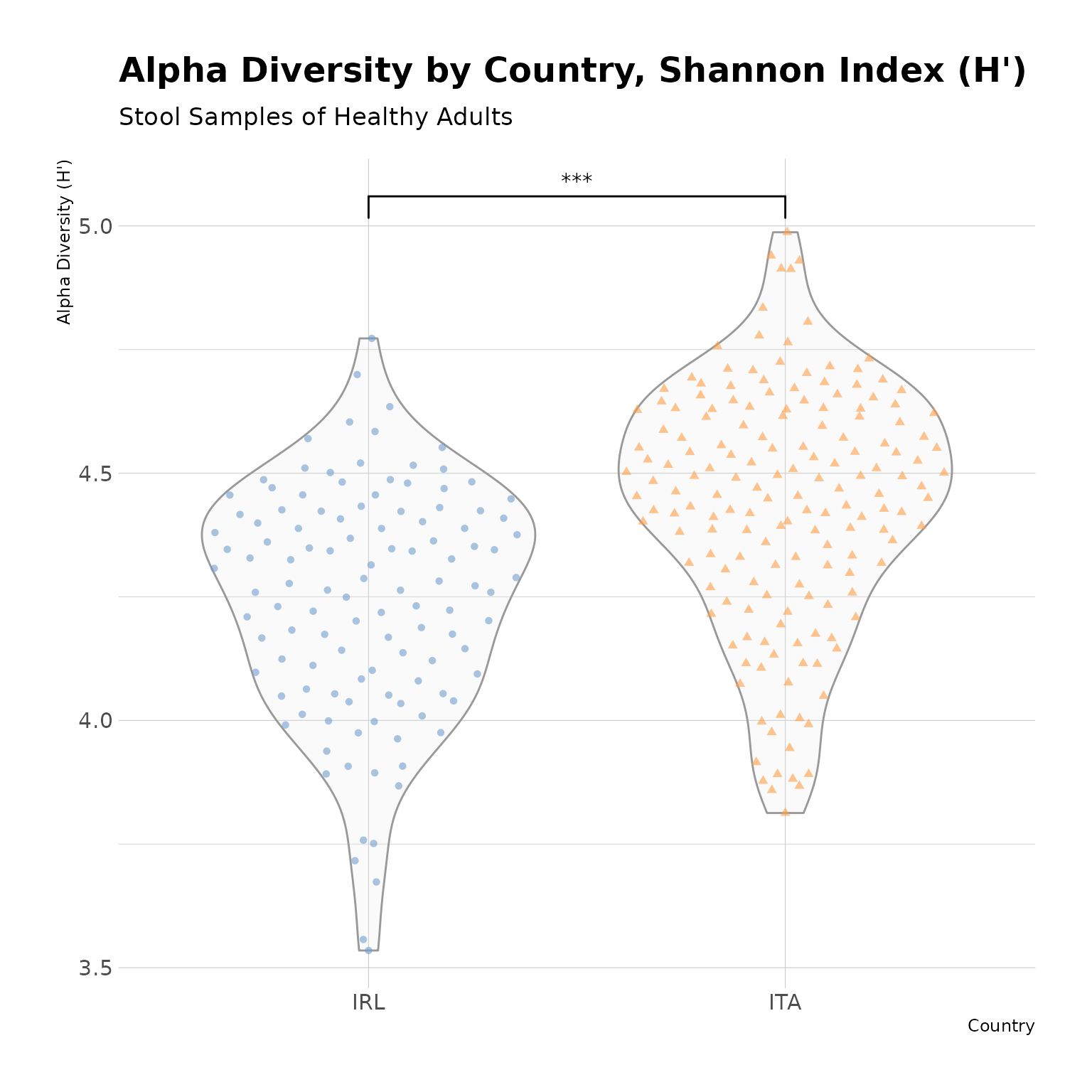

Alpha Diversity by Country. Alpha Diversity of stool samples from healthy adults, as measured by the Shannon index (H’), is significantly $(Pr(T < t) < 0.001)$ lower among Irish samples, as compared to Italian samples.

Analysis of Beta Diversity

Beta diversity is a measurement of between sample variation that is usually qualitatively assessed using a low-dimensional embedding; classically this has been done in metagenomics with a principal coordinates analysis (PCoA) of Bray-Curtis dissimilarity.¹ This is done below using the runMDS() function from the scater package with the vegdist function from the vegan package. The plotReducedDim() function from the scater package is used to generate a basic ggplot2 plot, which is styled further.

countryData |>
  runMDS(FUN = vegdist, method = "bray", exprs_values = "logcounts", name = "BrayCurtis") |>
  plotReducedDim("BrayCurtis", colour_by = "country", shape_by = "country", text_by = "country") +
  labs(
    title = "Beta Diversity by Country, Bray-Curtis PCoA",
    subtitle = "Stool Samples of Healthy Adults",
    x = "PCo 1",
    y = "PCo 2"
  ) +
  guides(color = guide_none(), shape = guide_none()) +
  theme_minimal()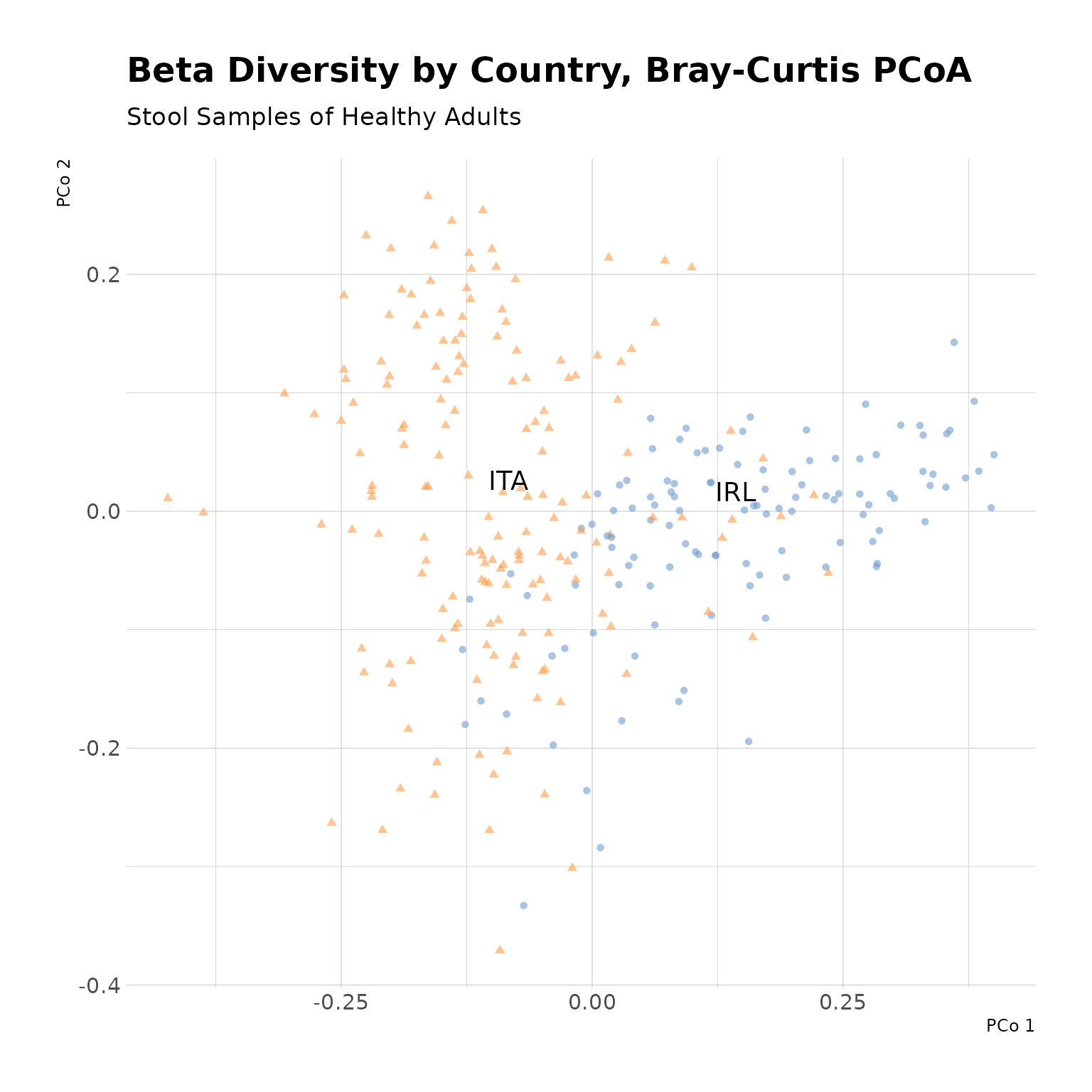

Beta Diversity by Country, Bray-Curtis PCoA. The first two principal coordinates demonstrate good seperation of Irish and Italian stool samples from healthy adults, suggesting differences in gut microbial composition between the two populations.

To address the issue of using principal coordinates analysis (PCoA) with a dissimilarity, beta diversity can be assessed using the UMAP (Uniform Manifold Approximation and Projection) algorithm instead.² The runUMAP() function from the scater package is used below; otherwise, the syntax is largely the same as above.

countryData |>
  runUMAP(exprs_values = "logcounts", name = "UMAP") |>
  plotReducedDim("UMAP", colour_by = "country", shape_by = "country", text_by = "country") +
  labs(
    title = "Beta Diversity by Country, UMAP Embedding",
    subtitle = "Stool Samples of Healthy Adults",
    x = "UMAP 1",
    y = "UMAP 2"
  ) +
  guides(color = guide_none(), shape = guide_none()) +
  theme_minimal()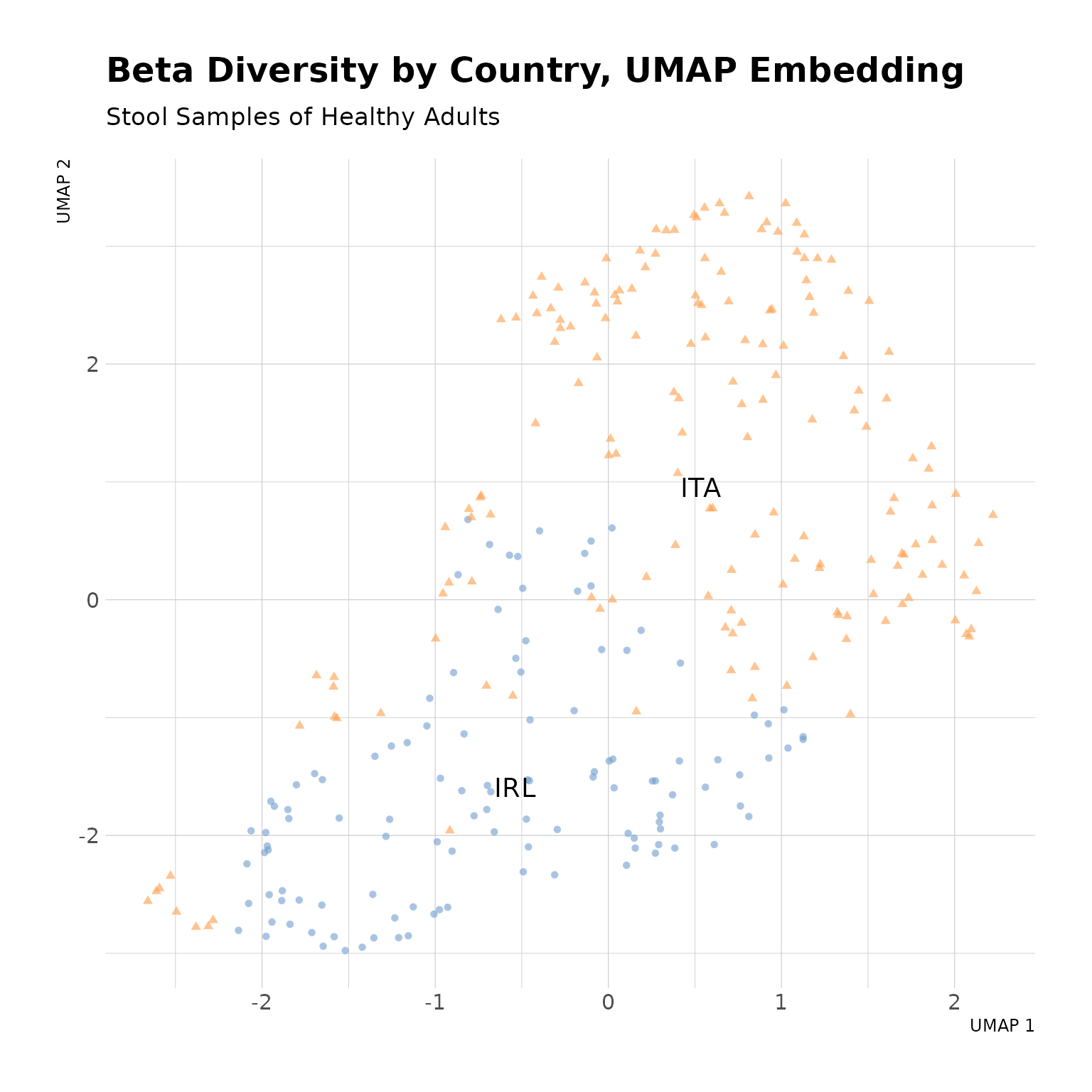

Beta Diversity by Country, UMAP Embedding. The two-dimensional UMAP embedding demonstrates good seperation of Irish and Italian stool samples from healthy adults, suggesting differences in gut microbial composition between the two populations.

Modeling Bacteria by Country

Where beta diversity embeddings suggest there are features that separate Irish and Italian stool samples from healthy adults, you might like to know which are most differentially abundance. To assess this the ANCOMBC package has a metagenomics-specific additive log-ratio model for the task. However, the ancombc() function requires a phyloseq class objects – one can be created using the makePhyloseqFromTreeSummarizedExperiment() function from the mia package, as shown below.

ancombcResults <-
  mia::convertToPhyloseq(countryData) |>
  ancombc(formula="country", group="country")

The results of the ANCOMBC model are in a strange list structure and have to be coerced into a data.frame before they can be displayed; the bind_cols() function from the dplyr package is used below.

# Extract the results for the country coefficient (countryITA)
ancombcTable <- data.frame(
  beta = ancombcResults$res$lfc$countryITA,
  se = ancombcResults$res$se$countryITA,
  p_val = ancombcResults$res$p_val$countryITA,
  q_val = ancombcResults$res$q_val$countryITA,
  row.names = rownames(ancombcResults$feature_table)
)

The row names of the results table are big long strings of microbial taxonomies that will need some editing if they are to be displayed nicely. the rownames_to_column() function from the tibble package is used below to turn them into a column so they can be edited.

ancombcTable <- rownames_to_column(ancombcTable)

Before the row names are split into 7 pieces, the names of columns that each piece will be assigned to are created below.

rankNames <-
  c("Kingdom", "Phylum", "Class", "Order", "Family", "Genus", "Species")

The row names of the results table are then transformed using tidyr, dplyr, and stringr, as shown below.

ancombcTable[["rowname"]] <-
  separate(ancombcTable, rowname, rankNames, sep = "\\|") |>
  select(all_of(rankNames)) |>
  mutate(across(everything(), ~ str_remove_all(.x, ".__"))) |>
  mutate(across(everything(), ~ str_replace_all(.x, "_", " "))) |>
  mutate(label = Species) |>
  pull(label)

Once the results table is in good shape, it can be filtered to include only bacterial species that exhibited large (e.g. abs(beta) > 1) and significant (-log10(q_val) > 5) differences in abundances between the two countries. In the example below, the table is sorted by effect size and a number of formatting conventions are applied before displaying the results table.

filter(ancombcTable, abs(beta) > 1) |>
  filter(-log10(q_val) > 5) |>
  select(rowname, beta, se, p_val, q_val) |>
  arrange(-abs(beta)) |>
  column_to_rownames() |>
  mutate(across(everything(), .fns = ~ round(.x, digits = 3))) |>
  mutate(beta = format(beta)) |>
  mutate(beta = str_replace(beta, " ", "&nbsp;")) |>
  mutate(p_val = if_else(p_val == 0, "< 0.001", format(p_val, nsmall = 3))) |>
  mutate(q_val = if_else(q_val == 0, "< 0.001", format(q_val, nsmall = 3))) |>
  kable(col.names = c("β", "SE", "P", "Q"), align = "cccc", escape = FALSE)

	β	SE	P	Q
Catenibacterium mitsuokai	-8.872	0.615	< 0.001	< 0.001
Holdemanella biformis	-8.159	0.574	< 0.001	< 0.001
Eubacterium sp CAG 180	-7.331	0.694	< 0.001	< 0.001
Bacteroides dorei	6.269	0.558	< 0.001	< 0.001
Lactobacillus ruminis	-6.088	0.562	< 0.001	< 0.001
Phascolarctobacterium succinatutens	-5.970	0.712	< 0.001	< 0.001
Ruminococcus torques	-5.703	0.450	< 0.001	< 0.001
Alistipes putredinis	5.690	0.624	< 0.001	< 0.001
Eubacterium hallii	-5.384	0.444	< 0.001	< 0.001
Bifidobacterium angulatum	-5.301	0.549	< 0.001	< 0.001
Prevotella sp CAG 279	-5.122	0.630	< 0.001	< 0.001
Dorea formicigenerans	-4.970	0.374	< 0.001	< 0.001
Lawsonibacter asaccharolyticus	4.946	0.413	< 0.001	< 0.001
Methanobrevibacter smithii	-4.735	0.640	< 0.001	< 0.001
Prevotella sp 885	-4.697	0.590	< 0.001	< 0.001
Coprococcus comes	-4.589	0.424	< 0.001	< 0.001
Oscillibacter sp CAG 241	-4.478	0.546	< 0.001	< 0.001
Roseburia intestinalis	-4.462	0.566	< 0.001	< 0.001
Slackia isoflavoniconvertens	-4.422	0.586	< 0.001	< 0.001
Eubacterium ramulus	-4.376	0.495	< 0.001	< 0.001
Ruminococcus callidus	-4.366	0.519	< 0.001	< 0.001
Coprococcus catus	-4.316	0.429	< 0.001	< 0.001
Intestinibacter bartlettii	-4.227	0.536	< 0.001	< 0.001
Eubacterium sp CAG 251	-3.925	0.657	< 0.001	< 0.001
Dorea longicatena	-3.896	0.332	< 0.001	< 0.001
Alistipes finegoldii	3.819	0.547	< 0.001	< 0.001
Prevotella sp AM42 24	-3.603	0.563	< 0.001	< 0.001
Roseburia faecis	-3.573	0.497	< 0.001	< 0.001
Firmicutes bacterium CAG 170	-3.390	0.582	< 0.001	< 0.001
Bacteroides plebeius	3.291	0.529	< 0.001	< 0.001
Alistipes shahii	3.248	0.535	< 0.001	< 0.001
Bacteroides eggerthii	3.135	0.483	< 0.001	< 0.001
Parasutterella excrementihominis	3.117	0.485	< 0.001	< 0.001
Blautia wexlerae	-3.111	0.434	< 0.001	< 0.001
Eubacterium rectale	-3.084	0.413	< 0.001	< 0.001
Parabacteroides distasonis	3.069	0.530	< 0.001	< 0.001
Clostridium disporicum	-3.037	0.443	< 0.001	< 0.001
Butyricimonas virosa	3.035	0.462	< 0.001	< 0.001
Alistipes indistinctus	2.945	0.522	< 0.001	< 0.001
Anaerostipes hadrus	-2.895	0.463	< 0.001	< 0.001
Bacteroides sp CAG 530	-2.847	0.413	< 0.001	< 0.001
Blautia obeum	-2.833	0.410	< 0.001	< 0.001
Intestinimonas butyriciproducens	2.698	0.469	< 0.001	< 0.001
Roseburia inulinivorans	-2.586	0.369	< 0.001	< 0.001
Prevotella stercorea	-2.571	0.460	< 0.001	< 0.001
Collinsella aerofaciens	-2.364	0.323	< 0.001	< 0.001
Fusicatenibacter saccharivorans	-1.571	0.274	< 0.001	< 0.001

While the table above is somewhat interesting, the results are better summarized as a volcano plot (i.e. statistical significance versus fold change) and one can be made using the results table. To shorten labels for readability, stringr is first used to abbreviate species names by replacing the first word of the name with a single letter followed by a period. Next, the same filtering of the table as above is undertaken, and the color scheme used in all the plots above is applied. Both labeling and coloring are only applied where effect size and significance thresholds are met, as denoted by the dotted lines.

ancombcTable |>
  mutate(rowname = str_replace(rowname, "^([A-Z])([a-z])+ ", "\\1. ")) |>
  mutate(q_val = -log10(q_val)) |>
  mutate(label = if_else(abs(beta) > 1, rowname, NA_character_)) |>
  mutate(label = if_else(q_val > 5, label, NA_character_)) |>
  mutate(color = if_else(beta > 0, "#FF9E4A", "#729ECE")) |>
  mutate(color = if_else(is.na(label), "#000000", color)) |>
  ggplot(mapping = aes(beta, q_val, color = I(color), label = label, shape = I(1))) +
  geom_point() +
  geom_hline(linetype = "dotted", yintercept = 5) +
  geom_vline(linetype = "dotted", xintercept = 1) +
  geom_vline(linetype = "dotted", xintercept = -1) +
  geom_label_repel(min.segment.length = 0, force = 10, max.overlaps = 20, na.rm = TRUE) +
  labs(
    title = "Significance vs. Effect Size, ANCOM-BC",
    subtitle = "Stool Samples of Healthy Adults",
    x = expression(beta),
    y = expression(-~log[10]~Q)
  ) +
  guides(color = guide_none(), shape = guide_none()) +
  theme_minimal()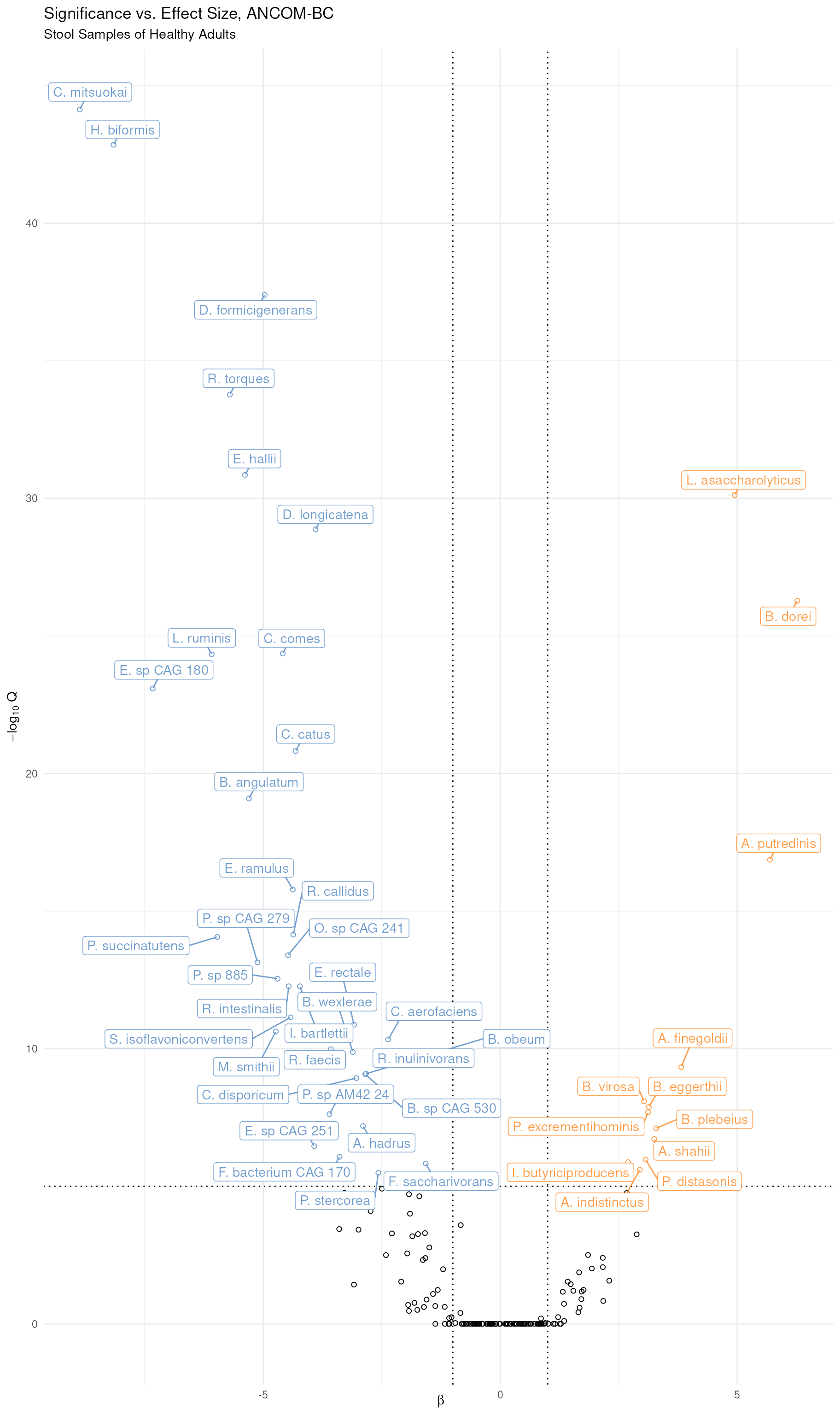

Volcano Plot of Differentially Abundance Bacterial Species. In the model and the figure, Irish samples are the reference group such that bacterial species in blue at the left are significantly more abundant in Irish samples and those in yellow at the right are significantly more abundant in Italian samples.

As a bonus, do a Google or a PubMed search for Holdemanella biformis to see what condition(s) it is associated with and then explore differences between the two countries using GBD Compare visualizations.

Lucas Schiffer, MPH

October 6, 2021