Applied Statistics for High-throughput Biology: Session 2

Schematic of a typical scRNA-seq analysis workflow

Single-cell workflow

Each stage (separated by dashed lines) consists of a number of specific steps, many of which operate on and modify a SingleCellExperiment instance. (original image)

Day 4 outline

Book chapter 8:

Distances in high dimensions
Principal Components Analysis and Singular Value Decomposition
Multidimensional Scaling
t-SNE and UMAP

Metrics and distances

A metric satisfies the following five properties:

non-negativity \(d(a, b) \ge 0\)
symmetry \(d(a, b) = d(b, a)\)
identification mark \(d(a, a) = 0\)
definiteness \(d(a, b) = 0\) if and only if \(a=b\)
triangle inequality \(d(a, b) + d(b, c) \ge d(a, c)\)

A distance is only required to satisfy 1-3.
A similarity function satisfies 1-2, and increases as \(a\) and \(b\) become more similar
A dissimilarity function satisfies 1-2, and decreases as \(a\) and \(b\) become more similar

Euclidian distance (metric)

Remember grade school: Euclidean d = \(\sqrt{ (A_x-B_x)^2 + (A_y-B_y)^2}\).
Side note: also referred to as \(L_2\) norm

Euclidian distance in high dimensions

## BiocManager::install("genomicsclass/tissuesGeneExpression") #if needed
## BiocManager::install("genomicsclass/GSE5859") #if needed
library(GSE5859)
library(tissuesGeneExpression)
data(tissuesGeneExpression)
dim(e) ##gene expression data
#> [1] 22215   189
table(tissue) ##tissue[i] corresponds to e[,i]
#> tissue
#>  cerebellum       colon endometrium hippocampus      kidney       liver 
#>          38          34          15          31          39          26 
#>    placenta 
#>           6

Interested in identifying similar samples and similar genes

Notes about Euclidian distance in high dimensions

Points are no longer on the Cartesian plane
instead they are in higher dimensions. For example:
- sample \(i\) is defined by a point in 22,215 dimensional space: \((Y_{1,i},\dots,Y_{22215,i})^\top\).
- feature \(g\) is defined by a point in 189 dimensions \((Y_{g,189},\dots,Y_{g,189})^\top\)

Euclidean distance as for two dimensions. E.g., the distance between two samples \(i\) and \(j\) is:

\[ \mbox{dist}(i,j) = \sqrt{ \sum_{g=1}^{22215} (Y_{g,i}-Y_{g,j })^2 } \]

and the distance between two features \(h\) and \(g\) is:

\[ \mbox{dist}(h,g) = \sqrt{ \sum_{i=1}^{189} (Y_{h,i}-Y_{g,i})^2 } \]

Euclidian distance in matrix algebra notation

The Euclidian distance between samples \(i\) and \(j\) can be written as:

\[ \mbox{dist}(i,j) = \sqrt{ (\mathbf{Y}_i - \mathbf{Y}_j)^\top(\mathbf{Y}_i - \mathbf{Y}_j) }\]

with \(\mathbf{Y}_i\) and \(\mathbf{Y}_j\) columns \(i\) and \(j\).

t(matrix(1:3, ncol = 1))
#>      [,1] [,2] [,3]
#> [1,]    1    2    3
matrix(1:3, ncol = 1)
#>      [,1]
#> [1,]    1
#> [2,]    2
#> [3,]    3
t(matrix(1:3, ncol = 1)) %*% matrix(1:3, ncol = 1)
#>      [,1]
#> [1,]   14

Note about matrix algebra in R

R is very efficient at matrix algebra
for very large matricies, see the:
- Matrix CRAN package (sparse matrices)
- rhdf5 and DelayedArray Bioconductor package (on-disk arrays)

3 sample example

kidney1 <- e[, 1]
kidney2 <- e[, 2]
colon1 <- e[, 87]
sqrt(sum((kidney1 - kidney2) ^ 2))
#> [1] 85.8546
sqrt(sum((kidney1 - colon1) ^ 2))
#> [1] 122.8919

3 sample example using dist()

dim(e)
#> [1] 22215   189
(d <- dist(t(e[, c(1, 2, 87)])))
#>                 GSM11805.CEL.gz GSM11814.CEL.gz
#> GSM11814.CEL.gz         85.8546                
#> GSM92240.CEL.gz        122.8919        115.4773
class(d)
#> [1] "dist"

The dist() function

Excerpt from ?dist:

dist(
    x,
    method = "euclidean",
    diag = FALSE,
    upper = FALSE,
    p = 2
)

method: the distance measure to be used.
- This must be one of “euclidean”, “maximum”, “manhattan”, “canberra”, “binary” or “minkowski”. Any unambiguous substring can be given.
dist class output from dist() is used for many clustering algorithms and heatmap functions

Caution: dist(e) creates a 22215 x 22215 matrix that will probably crash your R session.

Note on standardization

In practice, features (e.g. genes) are typically “standardized”, i.e. converted to z-score:

\[x_{gi} \leftarrow \frac{(x_{gi} - \bar{x}_g)}{s_g}\]

This is done because the differences in overall levels between features are often not due to biological effects but technical ones, e.g.:
- GC bias, PCR amplification efficiency, …
Euclidian distance and \(1-r\) (Pearson cor) are related:
- \(\frac{d_E(x, y)^2}{2m} = 1 - r_{xy}\)
- \(m\) = # dimensions

Dimension reduction and PCA

Motivation for dimension reduction

Simulate the heights of twin pairs:

set.seed(1)
n <- 100
y <- t(MASS::mvrnorm(n, c(0, 0), matrix(c(1, 0.95, 0.95, 1), 2, 2)))
dim(y)
#> [1]   2 100
cor(t(y))
#>           [,1]      [,2]
#> [1,] 1.0000000 0.9433295
#> [2,] 0.9433295 1.0000000

Visualizing twin pairs data

Not much distance is lost in the second dimension

Not much loss of height differences when just using average heights of twin pairs.
- because twin heights are highly correlated

Singular Value Decomposition (SVD)

SVD generalizes the example rotation we looked at:

\[\mathbf{Y} = \mathbf{UDV}^\top\]

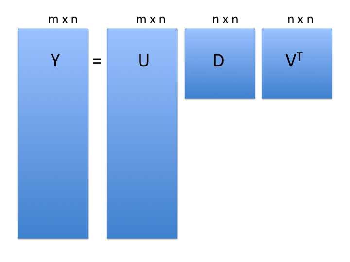
note: the above formulation is for \(m\) rows \(> n\) columns
\(\mathbf{Y}\): the \(m\) rows x \(n\) cols matrix of measurements
\(\mathbf{U}\): \(m \times n\) matrix relating original scores to PCA scores (loadings)
\(\mathbf{D}\): \(n \times n\) diagonal matrix (eigenvalues)
\(\mathbf{V}\): \(n \times n\) orthogonal matrix (eigenvectors or PCA scores)
- orthogonal = unit length and “perpendicular” in 3-D

SVD of gene expression dataset

Scaling:

e.standardize <- t(scale(t(e), scale = FALSE))

SVD:

s <- svd(e.standardize)
names(s)
#> [1] "d" "u" "v"

Components of SVD results

dim(s$u)     # loadings
#> [1] 22215   189
length(s$d)  # eigenvalues
#> [1] 189
dim(s$v)     # d %*% vT = scores
#> [1] 189 189

PCA is a SVD

gene expression dataset

rafalib::mypar()
p <- prcomp(t(e.standardize))
plot(s$u[, 1] ~ p$rotation[, 1])

Lesson: u and v can each be multiplied by -1 arbitrarily

PCA interpretation: loadings

\(\mathbf{U}\) (loadings): relate the principal component axes to the original variables
- think of principal component axes as a weighted combination of original axes

Visualizing PCA loadings

plot(p$rotation[, 1],
     xlab = "Index of genes",
     ylab = "Loadings of PC1",
     main = "PC1 loadings of each gene") #or, predict(p)
abline(h = c(-0.03, 0.03), col = "red")

Genes with high PC1 loadings

e.pc1genes <-
    e.standardize[p$rotation[, 1] < -0.03 |
                           p$rotation[, 1] > 0.03,]
pheatmap::pheatmap(
    e.pc1genes,
    scale = "none",
    show_rownames = TRUE,
    show_colnames = FALSE
)

PCA interpretation: eigenvalues

\(\mathbf{D}\) (eigenvalues): standard deviation scaling factor that each decomposed variable is multiplied by.

rafalib::mypar()
plot(
    p$sdev ^ 2 / sum(p$sdev ^ 2) * 100,
    xlim = c(0, 150),
    type = "b",
    ylab = "% variance explained",
    main = "Screeplot"
)

PCA interpretation: eigenvalues

Alternatively as cumulative % variance explained (using cumsum() function)

rafalib::mypar()
plot(
    cumsum(p$sdev ^ 2) / sum(p$sdev ^ 2) * 100,
    ylab = "cumulative % variance explained",
    ylim = c(0, 100),
    type = "b",
    main = "Cumulative screeplot"
)

PCA interpretation: scores

\(\mathbf{V}\) (scores): The “datapoints” in the reduced prinipal component space
In some implementations (like prcomp()), scores are already scaled by eigenvalues: \(\mathbf{D V^T}\)

PCA interpretation: scores

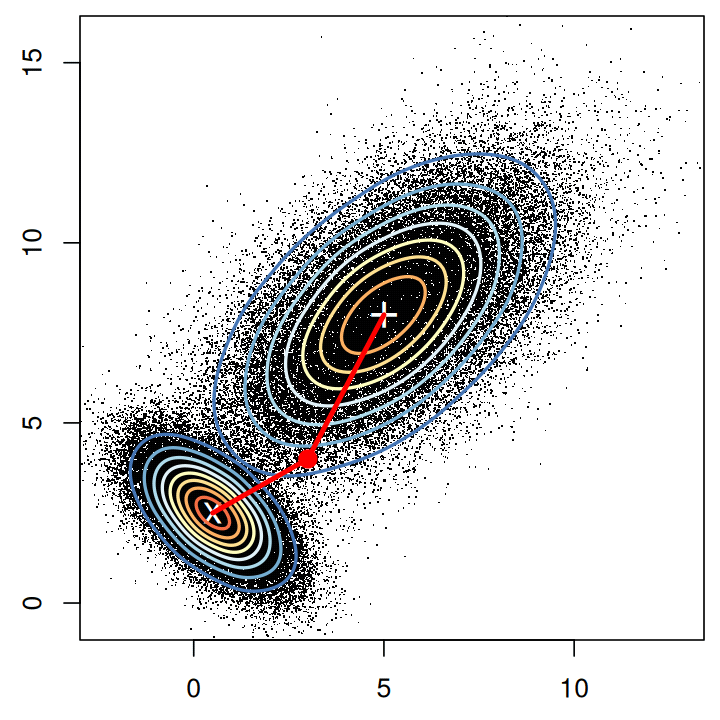
Multi-dimensional Scaling (MDS)

also referred to as Principal Coordinates Analysis (PCoA)
a reduced SVD, performed on a distance matrix
identify two (or more) eigenvalues/vectors that preserve distances

d <- as.dist(1 - cor(e.standardize))
mds <- cmdscale(d)

t-SNE

non-linear dimension reduction method very popular for visualizing single-cell data
- almost magical ability to show clearly separated clusters
- performs different transformations on different regions
computationally intensive so usually done only on top ~30 PCs
t-SNE is sensitive to choices of tuning parameters
- “perplexity” parameter defines (loosely) how to balance attention between local and global aspects of data
- optimal choice of perplexity changes for different numbers of cells from the same sample.
- perplexity = \(\sqrt{N}\) is one rule of thumb. \(max(N/5, 50)\) is another (default of Rtsne)
- Here is a good post by Nikolay Oskolkov on this topic.

t-SNE caveats

uses a random number generator
apparent spread of clusters is completely meaningless
distance between clusters might also not mean anything
parameters can be tuned to make data appear how you want
can show apparent clusters in random noise. Should not be used for statistical inference
Try it to gain some intuition: https://distill.pub/2016/misread-tsne/)

tSNE

PCA of Zeisel single-cell RNA-seq dataset

sce.zeisel <- fixedPCA(sce.zeisel, subset.row=NULL)
plotReducedDim(sce.zeisel, dimred="PCA", colour_by="level1class")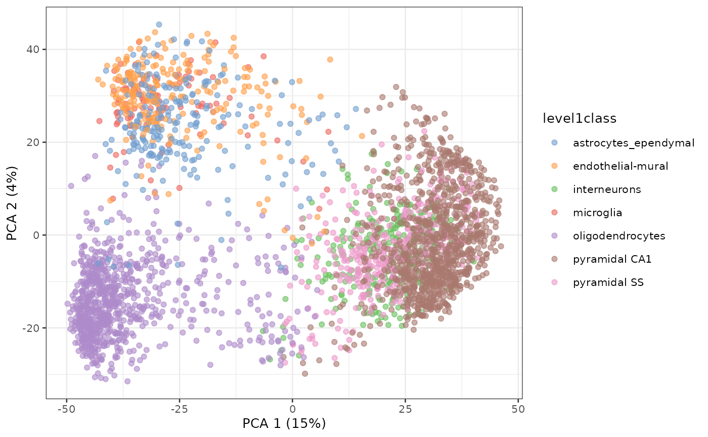

Principal Components Analysis of Zeisel dataset

t-SNE of the same dataset

sce.zeisel <- runTSNE(sce.zeisel, dimred="PCA")
plotReducedDim(sce.zeisel, dimred="TSNE", colour_by="level1class")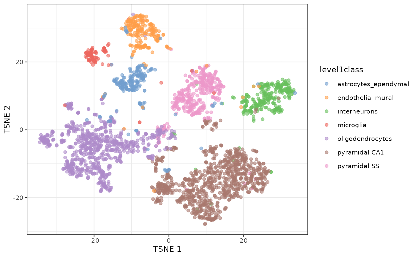

t-SNE clustering of Zeisel dataset

UMAP vs t-SNE

UMAP may better preserve local and global distances
tends to have more compact visual clusters with more empty space between them
more computationally efficient
also involves random number generation
Note: I prefer not setting the random number seed during exploratory analysis in order to see the random variability

UMAP of the same dataset

sce.zeisel <- runUMAP(sce.zeisel, dimred="PCA")
plotReducedDim(sce.zeisel, dimred="UMAP", colour_by="level1class")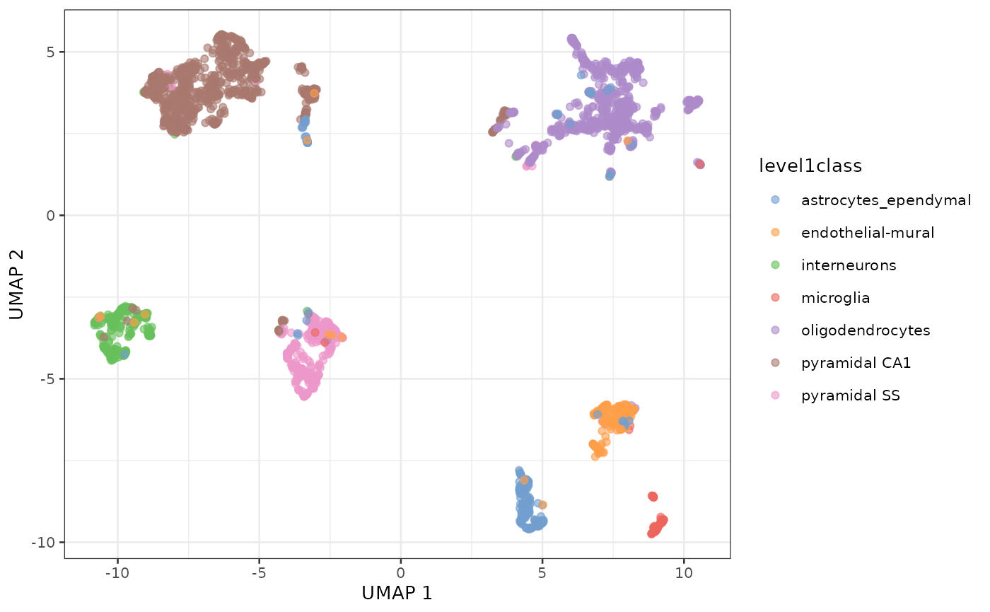

UMAP representation of the Zeisel dataset

tSNE of tissue microarray data

Using default parameters and no log transformation

sct <- SingleCellExperiment(e)
sct$tissue <- tissue
# fake the log normalization because it is undesirable for microarray data
names(assays(sct)) <- "logcounts" 
sct <- fixedPCA(sct, subset.row=NULL)
sct <- runTSNE(sct, dimred="PCA")
plotReducedDim(sct, dimred="TSNE", colour_by="tissue")

UMAP of tissue microarray data

Also using default parameters and no log transformation

sct <- runUMAP(sct, dimred="PCA")
plotReducedDim(sct, dimred="UMAP", colour_by="tissue")

Summary: distances and dimension reduction

Note: signs of eigenvalues (square to get variances) and eigenvectors (loadings) can be arbitrarily flipped
PCA and MDS are useful for dimension reduction when you have correlated variables
Variables are always centered.
Variables are also scaled unless you know they have the same scale in the population
PCA projection can be applied to new datasets if you know the matrix calculations
PCA is subject to over-fitting, screeplot can be tested by cross-validation
PCA is often used prior to t-SNE and UMAP for de-noising and computational tractability

Lab exercise

OSCA Basics: Chapter 4 Dimensionality Reduction
Optional if you are interested, OSCA Advanced: Chapter 4 Dimensionality reduction, redux

Levi Waldron

Schematic of a typical scRNA-seq analysis workflow

Day 4 outline

Metrics and distances

Euclidian distance (metric)

Euclidian distance in high dimensions

Notes about Euclidian distance in high dimensions

Euclidian distance in matrix algebra notation

Note about matrix algebra in R

3 sample example

3 sample example using dist()

The dist() function

Note on standardization

Dimension reduction and PCA

Visualizing twin pairs data

Not much distance is lost in the second dimension

Singular Value Decomposition (SVD)

SVD of gene expression dataset

Components of SVD results

PCA is a SVD

PCA interpretation: loadings

Visualizing PCA loadings

Genes with high PC1 loadings

PCA interpretation: eigenvalues

PCA interpretation: eigenvalues

PCA interpretation: scores

PCA interpretation: scores

Multi-dimensional Scaling (MDS)

t-SNE

t-SNE caveats

PCA of Zeisel single-cell RNA-seq dataset

t-SNE of the same dataset

UMAP vs t-SNE

UMAP of the same dataset

tSNE of tissue microarray data

UMAP of tissue microarray data

Summary: distances and dimension reduction

Lab exercise

Links