Applied Statistics for High-throughput Biology: Session 3

Levi Waldron

Outline

• Multiple linear regression
  • Continuous and categorical predictors
  • Interactions
• Model formulae
• Generalized Linear Models
  • Linear, logistic, log-Linear links
  • Poisson, Negative Binomial error distributions
• Multiple Hypothesis Testing

Textbook sources

• Biomedical Data Science
  • Chapter 5: Linear models
  • Chapter 6: Inference for high-dimensional data
• Modern Statistics for Modern Biology
  • Chapter 6: Testing
• OSCA multi-sample
  • Chapter 4: DE analyses between conditions

Example: friction of spider legs

• (A) Barplot showing total claw tuft area of the corresponding legs.
• (B) Boxplot presenting friction coefficient data illustrating median, interquartile range and extreme values.

• Wolff & Gorb, Radial arrangement of Janus-like setae permits friction control in spiders, Sci. Rep.

Questions

• Are the pulling and pushing friction coefficients different?
• Are the friction coefficients different for the different leg pairs?
• Does the difference between pulling and pushing friction coefficients vary by leg pair?

Qualitative answers

table(spider$leg,spider$type)
#>     
#>      pull push
#>   L1   34   34
#>   L2   15   15
#>   L3   52   52
#>   L4   40   40
summary(spider)
#>      leg                type              friction     
#>  Length:282         Length:282         Min.   :0.1700  
#>  Class :character   Class :character   1st Qu.:0.3900  
#>  Mode  :character   Mode  :character   Median :0.7600  
#>                                        Mean   :0.8217  
#>                                        3rd Qu.:1.2400  
#>                                        Max.   :1.8400

boxplot(spider$friction ~ spider$type * spider$leg,
        col=c("grey90","grey40"), las=2,
        main="Friction coefficients of different leg pairs")

Notes:

• Pulling friction is higher
• Pulling (but not pushing) friction increases for further back legs (L1 -> 4)
• Variance isn’t constant

What are linear models?

The following are examples of linear models:

1. \(Y_i = \beta_0 + \beta_1 x_i + \varepsilon_i\) (simple linear regression)
2. \(Y_i = \beta_0 + \beta_1 x_i + \beta_2 x_i^2 + \varepsilon_i\) (quadratic regression)
3. \(Y_i = \beta_0 + \beta_1 x_i + \beta_2 \times 2^{x_i} + \varepsilon_i\) (\(2^{x_i}\) is a new transformed variable)

Multiple linear regression model

• Linear models can have any number of predictors
• Systematic part of model:

\[ E[y|x] = \beta_0 + \beta_1 x_1 + \beta_2 x_2 + ... + \beta_p x_p \]

• \(E[y|x]\) is the expected value of \(y\) given \(x\)
• \(y\) is the outcome, response, or dependent variable
• \(x\) is the vector of predictors / independent variables
• \(x_p\) are the individual predictors or independent variables
• \(\beta_p\) are the regression coefficients

Random part of model:

\(y_i = E[y_i|x_i] + \epsilon_i\)

Assumptions of linear models: \(\epsilon_i \stackrel{iid}{\sim} N(0, \sigma_\epsilon^2)\)

• Normal distribution
• Mean zero at every value of predictors
• Constant variance at every value of predictors
• Values that are statistically independent

Continuous predictors

• Coding: as-is, or may be scaled to unit variance (which results in adjusted regression coefficients)
• Interpretation for linear regression: An increase of one unit of the predictor results in this much difference in the continuous outcome variable

Binary predictors (2 levels)

• Coding: indicator or dummy variable (0-1 coding)
• Interpretation for linear regression: the increase or decrease in average outcome levels in the group coded “1”, compared to the reference category (“0”)
  • e.g. \(E(y|x) = \beta_0 + \beta_1 x\)
  • where x={ 1 if push friction, 0 if pull friction }

Multilevel categorical predictors (ordinal or nominal)

• Coding: \(K-1\) dummy variables for \(K\)-level categorical variable
• Comparisons with respect to a reference category, e.g. L1:
  • L2={1 if \(2^{nd}\) leg pair, 0 otherwise},
  • L3={1 if \(3^{nd}\) leg pair, 0 otherwise},
  • L4={1 if \(4^{th}\) leg pair, 0 otherwise}.
• R re-codes factors to dummy variables automatically.
• Dummy coding depends on the reference level

Model formulae in R

Model formulae tutorial

• regression functions in R such as aov(), lm(), glm(), and coxph() use a “model formula” interface.
• The formula determines the model that will be built (and tested) by the R procedure. The basic format is:

> response variable ~ explanatory variables

• The tilde means “is modeled by” or “is modeled as a function of.”

Regression with a single predictor

Model formula for simple linear regression:

> y ~ x

• where “x” is the explanatory (independent) variable
• “y” is the response (dependent) variable.

Return to the spider legs

Friction coefficient for leg type of first leg pair:

spider.sub <- dplyr::filter(spider, leg=="L1")
fit <- lm(friction ~ type, data=spider.sub)
summary(fit)
#> 
#> Call:
#> lm(formula = friction ~ type, data = spider.sub)
#> 
#> Residuals:
#>      Min       1Q   Median       3Q      Max 
#> -0.33147 -0.10735 -0.04941 -0.00147  0.76853 
#> 
#> Coefficients:
#>             Estimate Std. Error t value Pr(>|t|)    
#> (Intercept)  0.92147    0.03827  24.078  < 2e-16 ***
#> typepush    -0.51412    0.05412  -9.499  5.7e-14 ***
#> ---
#> Signif. codes:  0 '***' 0.001 '**' 0.01 '*' 0.05 '.' 0.1 ' ' 1
#> 
#> Residual standard error: 0.2232 on 66 degrees of freedom
#> Multiple R-squared:  0.5776, Adjusted R-squared:  0.5711 
#> F-statistic: 90.23 on 1 and 66 DF,  p-value: 5.698e-14

Regression on spider leg type

Regression coefficients for friction ~ type for first set of spider legs:

broom::tidy(fit)
#> # A tibble: 2 × 5
#>   term        estimate std.error statistic  p.value
#>   <chr>          <dbl>     <dbl>     <dbl>    <dbl>
#> 1 (Intercept)    0.921    0.0383     24.1  2.12e-34
#> 2 typepush      -0.514    0.0541     -9.50 5.70e-14

• How to interpret this table?
  • Coefficients for (Intercept) and typepush
  • Coefficients are t-distributed when assumptions are correct
  • Standard deviation in the estimates of each coefficient can be calculated (standard errors)

Interpretation of spider leg type coefficients

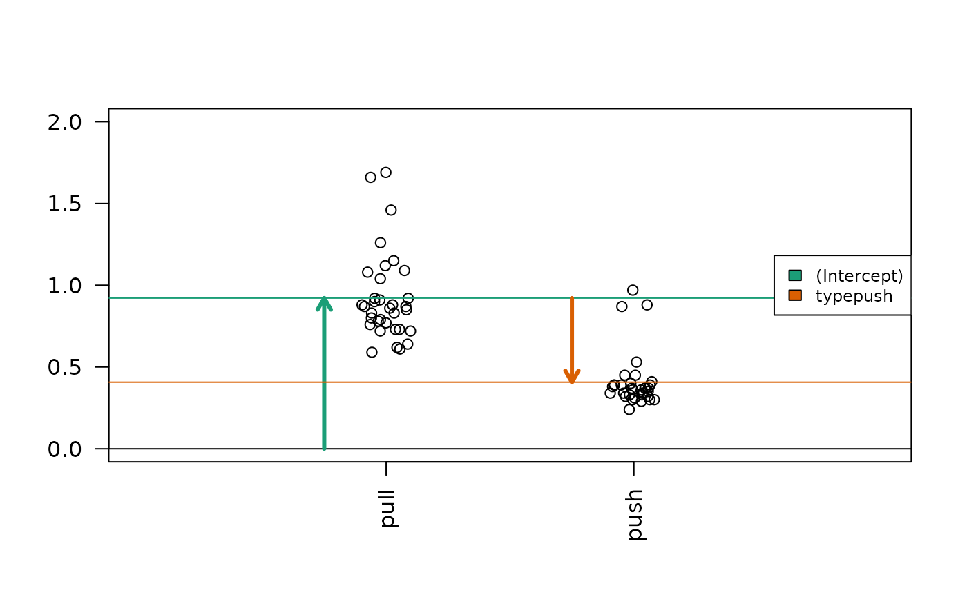
Diagram of the estimated coefficients in the linear model. The green arrow indicates the Intercept term, which goes from zero to the mean of the reference group (here the ‘pull’ samples). The orange arrow indicates the difference between the push group and the pull group, which is negative in this example. The circles show the individual samples, jittered horizontally to avoid overplotting.

regression on spider leg position

Remember there are positions 1-4

fit <- lm(friction ~ leg, data=spider)

fit.table <- xtable::xtable(fit, label=NULL)
print(fit.table, type="html")

	Estimate	Std. Error	t value	Pr(>|t|)
(Intercept)	0.6644	0.0538	12.34	0.0000
legL2	0.1719	0.0973	1.77	0.0784
legL3	0.1605	0.0693	2.32	0.0212
legL4	0.2813	0.0732	3.84	0.0002

• Interpretation of the dummy variables legL2, legL3, legL4 ?

Regression with multiple predictors

Additional explanatory variables can be added as follows:

> y ~ x + z

Note that “+” does not have its usual meaning, which would be achieved by:

> y ~ I(x + z)

Regression on spider leg type and position

Remember there are positions 1-4

fit <- lm(friction ~ type + leg, data=spider)

fit.table <- xtable::xtable(fit, label=NULL)
print(fit.table, type="html")

	Estimate	Std. Error	t value	Pr(>|t|)
(Intercept)	1.0539	0.0282	37.43	0.0000
typepush	-0.7790	0.0248	-31.38	0.0000
legL2	0.1719	0.0457	3.76	0.0002
legL3	0.1605	0.0325	4.94	0.0000
legL4	0.2813	0.0344	8.18	0.0000

• this model still doesn’t represent how the friction differences between different leg positions are modified by whether it is pulling or pushing

Interaction (effect modification)

Interaction is modeled as the product of two covariates: \[ E[y|x] = \beta_0 + \beta_1 x_1 + \beta_2 x_2 + \beta_{12} x_1*x_2 \]

Interaction between coffee and time of day on performance

Image credit: http://personal.stevens.edu/~ysakamot/

Model formulae (cont’d)

symbol	example	meaning
+	+ x	include this variable
-	- x	delete this variable
:	x : z	include the interaction
*	x * z	include these variables and their interactions
^	(u + v + w)^3	include these variables and all interactions up to three way
1	-1	intercept: delete the intercept

Note: order generally doesn’t matter (u+v OR v+u)

Summary: types of standard linear models

lm( y ~ u + v)

u and v factors: ANOVA
u and v numeric: multiple regression
one factor, one numeric: ANCOVA

• R does a lot for you based on your variable classes
  • be sure you know the classes of your variables
  • be sure all rows of your regression output make sense

Generalized Linear Models

• Linear regression is a special case of a broad family of models called “Generalized Linear Models” (GLM)
• This unifying approach allows to fit a large set of models using maximum likelihood estimation methods (MLE) (Nelder & Wedderburn, 1972)
• Can model many types of data directly using appropriate distributions, e.g. Poisson distribution for count data
• Transformations of \(y\) not needed

Components of a GLM

\[ g\left( E[y|x] \right) = \beta_0 + \beta_1 x_{1i} + \beta_2 x_{2i} + ... + \beta_p x_{pi} \]

• Random component specifies the conditional distribution for the response variable
  • doesn’t have to be normal
  • can be any distribution in the “exponential” family of distributions
• Systematic component specifies linear function of predictors (linear predictor)
• Link [denoted by \(g(.)\)] specifies the relationship between the expected value of the random component and the systematic component
  • can be linear or nonlinear

Linear Regression as GLM

• Useful for log-transformed microarray data

• The model: \(y_i = E[y|x] + \epsilon_i = \beta_0 + \beta_1 x_{1i} + \beta_2 x_{2i} + ... + \beta_p x_{pi} + \epsilon_i\)

• Random component of \(y_i\) is normally distributed: \(\epsilon_i \stackrel{iid}{\sim} N(0, \sigma_\epsilon^2)\)

• Systematic component (linear predictor): \(\beta_0 + \beta_1 x_{1i} + \beta_2 x_{2i} + ... + \beta_p x_{pi}\)

• Link function here is the identity link: \(g(E(y | x)) = E(y | x)\). We are modeling the mean directly, no transformation.

Logistic Regression as GLM

• Useful for binary outcomes, e.g. Single Nucleotide Polymorphisms or somatic variants

• The model: \[ Logit(P(x)) = log \left( \frac{P(x)}{1-P(x)} \right) = \beta_0 + \beta_1 x_{1i} + \beta_2 x_{2i} + ... + \beta_p x_{pi} \]

• Random component: \(y_i\) follows a Binomial distribution (outcome is a binary variable)

• Systematic component: linear predictor \[ \beta_0 + \beta_1 x_{1i} + \beta_2 x_{2i} + ... + \beta_p x_{pi} \]

• Link function: logit (log of the odds that the event occurs)

\[ g(P(x)) = logit(P(x)) = log\left( \frac{P(x)}{1-P(x)} \right) \]

\[ P(x) = g^{-1}\left( \beta_0 + \beta_1 x_{1i} + \beta_2 x_{2i} + ... + \beta_p x_{pi} \right) \]

Log-linear GLM

The systematic part of the GLM is:

\[ log\left( E[y|x] \right) = \beta_0 + \beta_1 x_{1i} + \beta_2 x_{2i} + ... + \beta_p x_{pi} + log(t_i) \]

• Common for count data
  • can account for differences in sequencing depth by an offset \(log(t_i)\)
  • guarantees non-negative expected number of counts
  • often used in conjunction with Poisson or Negative Binomial error models

Poisson error model

\[ f(k, \lambda) = e^{-\lambda} \frac{\lambda^k}{k!} \]

• where \(f\) is the probability of \(k\) events (e.g. # of reads counted), and
• \(\lambda\) is the mean number of events, so \(E[y|x]\)
• \(\lambda\) is also the variance of the number of events

Negative Binomial error model

• aka gamma–Poisson mixture distribution

\[ f(k, \lambda, \theta) = \frac{\Gamma(\frac{1 + \theta k}{\theta})}{k! \, \Gamma(\frac{1}{\theta})} \left(\frac{\theta m}{1+\theta m}\right)^k \left(1+\theta m\right)^\theta \quad\text{for }k = 0, 1, 2, \dotsc \]

• where \(f\) is still the probability of \(k\) events (e.g. # of reads counted),
• \(\lambda\) is still the mean number of events, so \(E[y|x]\)
• An additional dispersion parameter \(\theta\) is estimated:
  • \(\theta \rightarrow 0\): Poisson distribution
  • \(\theta \rightarrow \infty\): Gamma distribution
• The Poisson model can be considered as nested within the Negative Binomial model
• A likelihood ratio test comparing the two models is possible

Compare Poisson vs. Negative Binomial

• The Negative Binomial Distribution (dbinom()) has two parameters:
  1. # of trials n,
  2. probability of success p

Additive vs. multiplicative models

• Linear regression is an additive model
  • e.g. for two binary variables \(\beta_1 = 1.5\), \(\beta_2 = 1.5\).
  • If \(x_1=1\) and \(x_2=1\), this adds 3.0 to \(E(y|x)\)
• Logistic and log-linear models are multiplicative:
  • If \(x_1=1\) and \(x_2=1\), this adds 3.0 to \(log(\frac{P}{1-P})\)
  • Odds-ratio \(\frac{P}{1-P}\) increases 20-fold: \(exp(1.5+1.5)\) or \(exp(1.5) * exp(1.5)\)

Inference in high dimensions (many variables)

• Conceptually similar to what we have already done
  • \(Y_i\) expression of a gene, etc
• Just repeated many times, e.g.:
  • is the mean expression of a gene different between two groups (t-test)
  • is the mean expression of a gene different between any of several groups (1-way ANOVA)
  • do this simple analysis thousands of times
  • note: for small sample sizes, some Bayesian improvements can be made (i.e. limma, edgeR, DESeq2)
• It is in prediction and machine learning where \(Y\) is a label like patient outcome, and we can have high-dimensional predictors

Multiple testing

• When testing thousands of true null hypotheses with \(\alpha = 0.05\), you expect a 5% type I error rate
• What p-values are even smaller than you expect by chance from multiple testing?
• Two mainstream approaches for controlling type I error rate:

1. Family-wise error rate (e.g., Bonferroni correction).
   • Controlling FWER at 0.05 ensures that the probably of any type I errors is < 0.05.
2. False Discovery Rate (e.g., Benjamini-Hochberg correction)
   • Controlling FDR at 0.05 ensures that fraction of type I errors is < 0.05.
   • see MSMB Chapter 6 - testing

Benjamini-Hochberg FDR algorithm

Source: MSMB Chapter 6

1. order the p-values from \(m\) hypothesis tests in increasing order, \(p_1, \ldots, p_m\)
2. for some choice of \(\phi\) (our target FDR), find the largest value of that \(k\) that satisfies: \(p_k \leq \phi k/m\)
3. reject the hypotheses \(1, \ldots, k\)

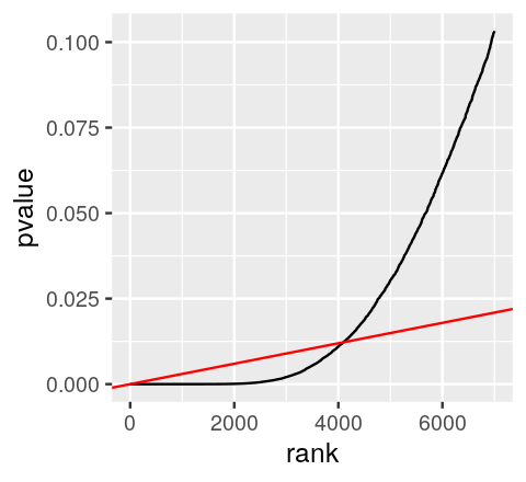
Benjamini-Hochberg FDR, visually

Important notes for intuition:

• You can have FDR < 0.05 with thousands of tests even if your smallest p-value is 0.01 or 0.001 (ie from permutation tests)
• FDR is a property of groups of tests, not of individual tests
• rank of FDR values can be different than rank of p-values

FDR alternatives to Benjamini-Hochberg

• “Local” False Discovery Rate or q-value
  • The q-value of a test estimates the proportion of false positives incurred when that particular test and all smaller p-values are called significant (packages: qvalue or fdrtool)
  • q-value increases monotonically with p-value (unlike Benjamini-Hochberg FDR)
• Independent Hypothesis Weighting
  • can improve power by modeling the relationship between a covariate property (such as mean expression) and probability of rejecting \(H_0\)
  • works best with lots of tests (ie, thousands)
  • implemented in the IHW Bioconductor package and in DESeq2

Beware of “double-dipping” in statistical inference

1. define a separation between observations
2. test for a difference across the separation

Example from: García-Mantrana et al., Gut Microbes 2020

• For a full treatment see https://arxiv.org/abs/2012.02936 and https://pubmed.ncbi.nlm.nih.gov/31521605
• Or a nice lecture: Daniela Whitten “Double-dipping” in statistics: https://youtu.be/tiv--XjPl9M

Simple example of double-dipping

Step 1: define an age classifier

• Elderly >70 yrs
• Youth <18 years
• Otherwise unclassified

Step 2: test for a difference in ages between elderly and youth

IMPORTANT: Even applying a fully-specified classifier to a validation dataset does not protect against inflated p-values from “double-dipping”

Summary

• Linear models are the basis for identifying differential expression / differential abundance

• Generalized Linear Models extend linear regression to:

  • binary \(y\) (logistic regression)
  • count \(y\) (log-linear regression with e.g. Poisson or Negative Binomial link functions)

• FWER, FDR, local FDR (q-value), Independent Hypothesis Testing

• Be aware of “double-dipping” in statistical inference

Exercises

• Repeat analyses of OSCA multi-sample Chapter 4: DE analyses between conditions

Please discuss the following questions:

1. What is a major problem with the hypothesis testing in 4.6 Testing for between-label differences?
   • (note, the inference problem is acknowledged in this section)
2. What is a related problem with the hypothesis testing in 4.4 Performing the DE analysis?
3. How might you avoid these same problems, with the same data or a multi’omic technology?

Links

• A built html version of this lecture is available.
• The source R Markdown is available from Github.