Summarization and quantitative trait analysis of CNV ranges
Vinicius Henrique da Silva
Luiz de Queiroz College of Agriculture, University of São PauloLudwig Geistlinger
Center for Computational Biomedicine, Harvard Medical SchoolSource:
vignettes/CNVRanger.Rmd
CNVRanger.RmdAbstract
The CNVRanger package implements a comprehensive tool suite for the analysis of copy number variation (CNV). This includes functionality for summarizing individual CNV calls across a population, assessing overlap with functional genomic regions, and association analysis with gene expression and quantitative phenotypes.
Report issues on https://github.com/waldronlab/CNVRanger/issues
Introduction
Copy number variation (CNV) is a frequently observed deviation from the diploid state due to duplication or deletion of genomic regions. CNVs can be experimentally detected based on comparative genomic hybridization, and computationally inferred from SNP-arrays or next-generation sequencing data. These technologies for CNV detection have in common that they report, for each sample under study, genomic regions that are duplicated or deleted with respect to a reference. Such regions are denoted as CNV calls in the following and will be considered the starting point for analysis with the CNVRanger package.
The following figure provides an overview of the analysis
capabilities of CNVRanger.
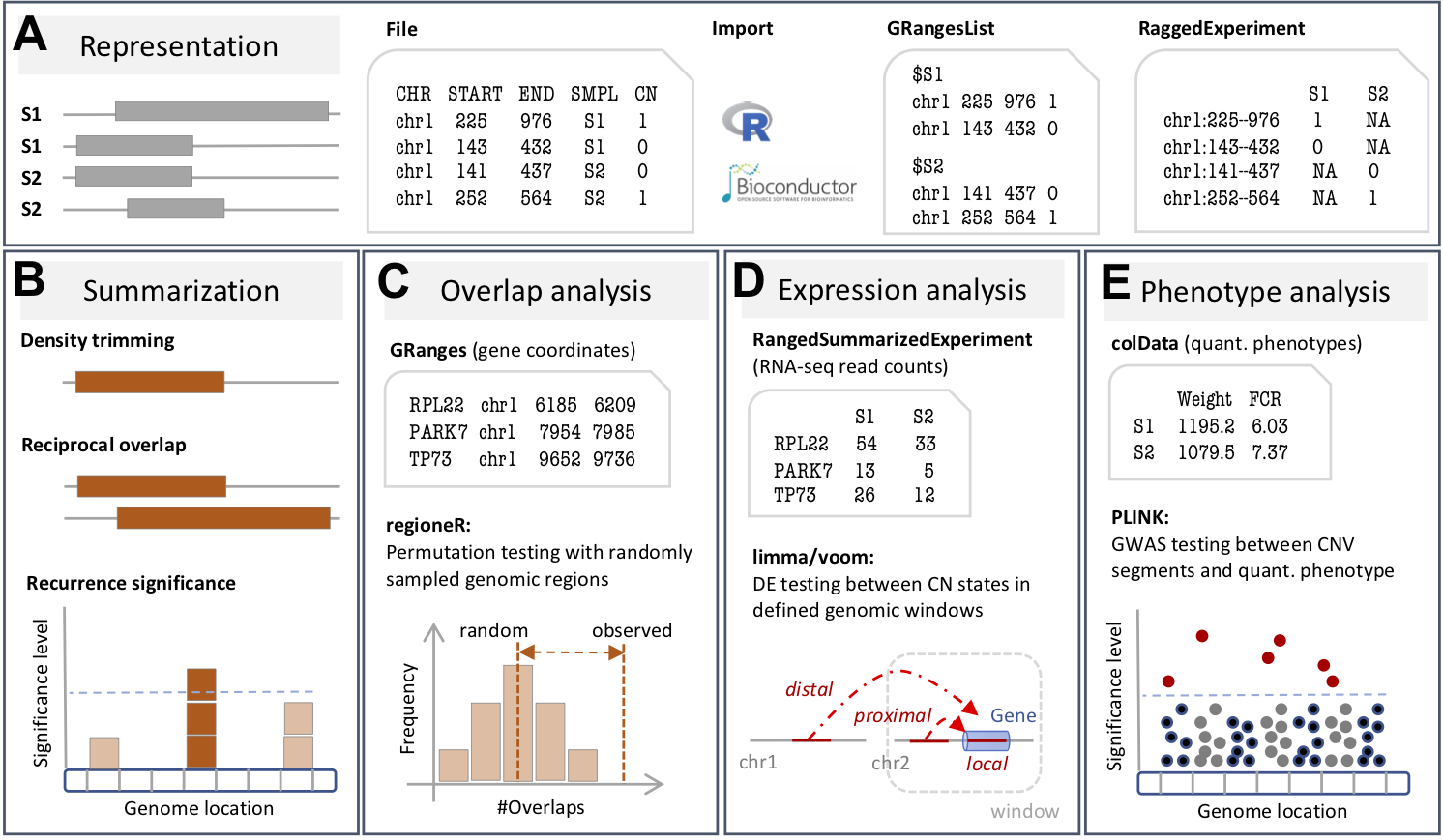
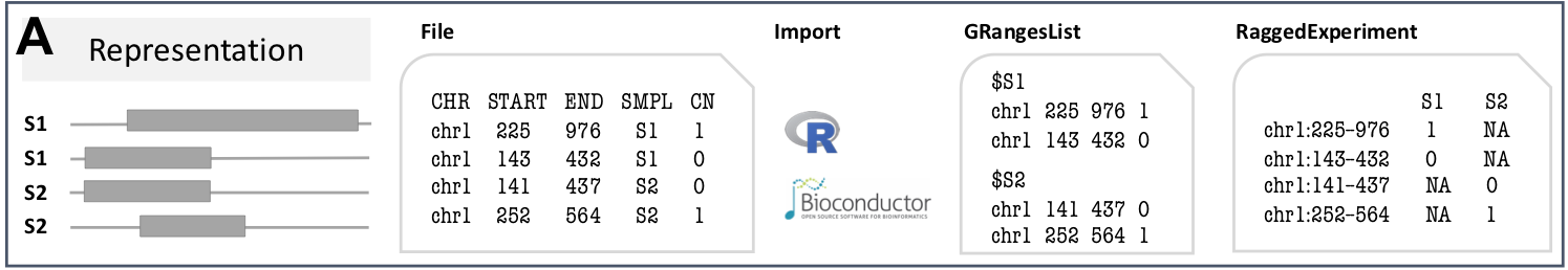
(A) The CNVRanger
package imports CNV calls from a simple file format into R,
and stores them in dedicated Bioconductor data structures, and
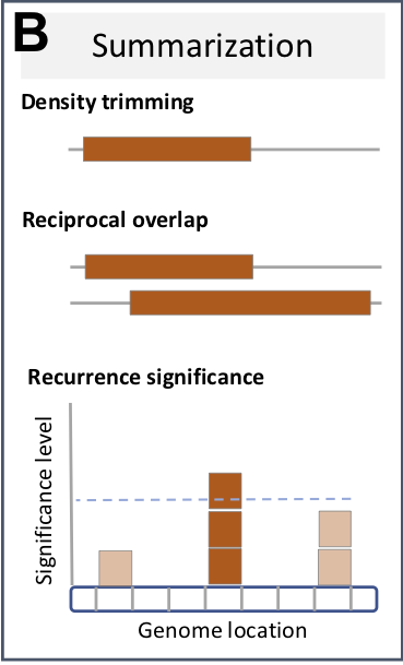
(B) implements three frequently used approaches for
summarizing CNV calls across a population: (i) the CNVRuler procedure that trims
region margins based on regional density (Kim et
al. 2012), (ii) the reciprocal overlap procedure that
requires sufficient mutual overlap between calls (Conrad et al. 2010), and (iii) the GISTIC
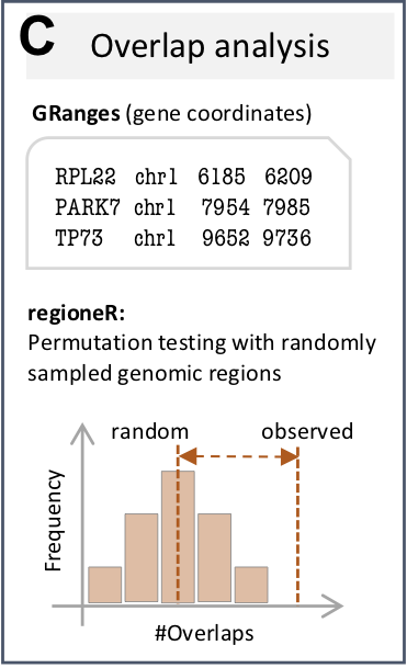
procedure that identifies recurrent CNV regions (Beroukhim et al. 2007). (C)
CNVRanger builds on regioneR
for overlap analysis of CNVs with functional genomic regions,
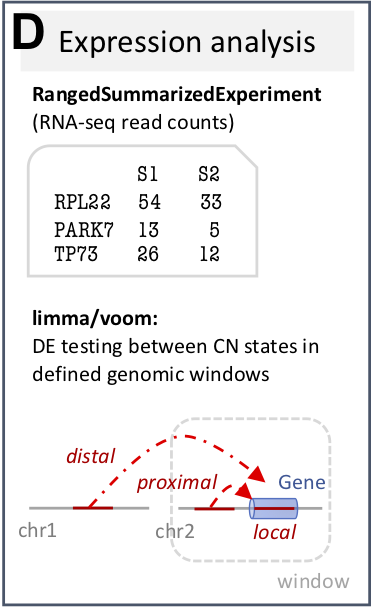
(D) implements RNA-seq expression Quantitative Trait
Loci (eQTL) analysis for CNVs by interfacing with edgeR, and
(E) performs linear regression for genome-wide
association studies (GWAS) that intend to link CNVs and quantitative
phenotypes.
The key parts of the functionality implemented in CNVRanger were developed, described, and applied in several previous studies:
Genome-wide detection of CNVs and their association with meat tenderness in Nelore cattle (Silva et al. 2016)
Widespread modulation of gene expression by copy number variation in skeletal muscle (Geistlinger et al. 2018)
CNVs are associated with genomic architecture in a songbird (Silva et al. 2018)
Applicability and Scope
As described in the above publications, CNVRanger
has been developed and extensively tested for SNP-based CNV calls as
obtained with PennCNV (Wang et al. 2007).
We also tested CNVRanger for sequencing-based CNV calls as
obtained with CNVnator (Abyzov et al.
2011) (a read-depth approach) or LUMPY (Layer et al. 2014) (an approach that combines
evidence from split-reads and discordant read-pairs).
In general, CNVRanger can be applied to CNV calls associated with integer copy number states, where we assume the states to be encoded as:
-
0: homozygous deletion (2-copy loss) -
1: heterozygous deletion (1-copy loss) -
2: normal diploid state -
3: 1-copy gain -
4: amplification (>= 2-copy gain)
Note that for CNV calling software that uses a different encoding or that does not provide integer copy number states, it is often possible to (at least approximately) transform the output to a format that is compatible with the input format of CNVRanger. See Section 4.1 Input data format for details.
CNVRanger is designed to work with CNV calls from one tool at a time. See EnsembleCNV (Zhang et al. 2019) and FusorSV (Becker et al. 2018) for combining CNV calls from multiple SNP-based callers or multiple sequencing-based callers, respectively.
CNVRanger assumes CNV calls provided as input to be already filtered by quality, using the software that was used for CNV calling, or specific tools for that purpose. CNVRanger provides downstream summarization and association analysis for CNV calls, it does not implement functions for CNV calling or quality control. CNVRanger is applicable for diploid species only.
Key functions
| Analysis step | Function |
|---|---|
| (A) Input | GenomicRanges::makeGRangesListFromDataFrame |
| (B) Summarization | populationRanges |
| (C) Overlap analysis | regioneR::overlapPermTest |
| (D) Expression analysis | cnvEQTL |
| (E) Phenotype analysis | cnvGWAS |
Note: we use the package::function notation for
functions from other packages. For functions from this package and base
R functions, we use the function name without preceding package
name.
Reading and accessing CNV data
The CNVRanger package uses Bioconductor core data structures implemented in the GenomicRanges and RaggedExperiment packages to efficiently represent, access, and manipulate CNV data.
We start by loading the package.
library(CNVRanger)Input data format
CNVRanger reads CNV calls from a simple file format, providing at least chromosome, start position, end position, sample ID, and integer copy number for each call.
For demonstration, we consider CNV calls as obtained with PennCNV from SNP-chip data in a Brazilian cattle breed (Silva et al. 2016).
Here, we use a data subset and only consider CNV calls on chromosome
1 and 2, for which there are roughly 3000 CNV calls as obtained for 711
samples. We use read.csv to read comma-separated values,
but we could use a different function if the data were provided with a
different delimiter (for example, read.delim for
tab-separated values).
data.dir <- system.file("extdata", package="CNVRanger")
call.file <- file.path(data.dir, "Silva16_PONE_CNV_calls.csv")
calls <- read.csv(call.file, as.is=TRUE)
nrow(calls)
## [1] 3000
head(calls)## chr start end NE_id state
## 1 chr1 16947 45013 NE001423 3
## 2 chr1 36337 67130 NE001426 3
## 3 chr1 16947 36337 NE001428 3
## 4 chr1 36337 105963 NE001519 3
## 5 chr1 36337 83412 NE001534 3
## 6 chr1 36337 83412 NE001648 3## [1] 711We observe that this example dataset satisfies the basic five-column input format required by CNVRanger.
The last column contains the integer copy number state for each call, encoded as
-
0: homozygous deletion (2-copy loss) -
1: heterozygous deletion (1-copy loss) -
2: normal diploid state -
3: 1-copy gain -
4: amplification (>= 2-copy gain)
For CNV detection software that uses a different encoding, it is necessary to convert to the above encoding. For example, GISTIC uses
-
-2: homozygous deletion (2-copy loss) -
-1: heterozygous deletion (1-copy loss) -
0: normal diploid state -
1: 1-copy gain -
2: amplification (>= 2-copy gain)
which can be converted by simply adding 2.
In Section 7.2 Application to TCGA data we also describe how to transform segmented log2 copy ratios to integer copy number states.
The basic five-column input format can be augmented with additional columns, providing additional characteristics and metadata for each CNV call. In Section 8 CNV-phenotype association analysis, we demonstrate how to make use of such an extended input format.
Representation as a GRangesList
Once read into an R data.frame, we group the calls by
sample ID and convert them to a GRangesList. Each element
of the list corresponds to a sample, and contains the genomic
coordinates of the CNV calls for this sample (along with the copy number
state in the state metadata column).
grl <- GenomicRanges::makeGRangesListFromDataFrame(calls,
    split.field="NE_id", keep.extra.columns=TRUE)
grl
## GRangesList object of length 711:
## $NE001357
## GRanges object with 5 ranges and 1 metadata column:
## seqnames ranges strand | state
## <Rle> <IRanges> <Rle> | <integer>
## [1] chr1 4569526-4577608 * | 3
## [2] chr1 15984544-15996851 * | 1
## [3] chr1 38306432-38330161 * | 3
## [4] chr1 93730576-93819471 * | 0
## [5] chr2 40529044-40540747 * | 3
## -------
## seqinfo: 2 sequences from an unspecified genome; no seqlengths
##
## $NE001358
## GRanges object with 1 range and 1 metadata column:
## seqnames ranges strand | state
## <Rle> <IRanges> <Rle> | <integer>
## [1] chr1 105042452-105233446 * | 1
## -------
## seqinfo: 2 sequences from an unspecified genome; no seqlengths
##
## $NE001359
## GRanges object with 4 ranges and 1 metadata column:
## seqnames ranges strand | state
## <Rle> <IRanges> <Rle> | <integer>
## [1] chr1 4569526-4577608 * | 3
## [2] chr1 31686841-31695808 * | 0
## [3] chr1 93730576-93819471 * | 0
## [4] chr2 2527718-2535261 * | 0
## -------
## seqinfo: 2 sequences from an unspecified genome; no seqlengths
##
## ...
## <708 more elements>The advantage of representing the CNV calls as a
GRangesList is that it allows to leverage the comprehensive
set of operations on genomic regions implemented in the GenomicRanges
packages - for instance, sorting of the calls according to their genomic
coordinates.
grl <- GenomicRanges::sort(grl)
grl
## GRangesList object of length 711:
## $NE001357
## GRanges object with 5 ranges and 1 metadata column:
## seqnames ranges strand | state
## <Rle> <IRanges> <Rle> | <integer>
## [1] chr1 4569526-4577608 * | 3
## [2] chr1 15984544-15996851 * | 1
## [3] chr1 38306432-38330161 * | 3
## [4] chr1 93730576-93819471 * | 0
## [5] chr2 40529044-40540747 * | 3
## -------
## seqinfo: 2 sequences from an unspecified genome; no seqlengths
##
## $NE001358
## GRanges object with 1 range and 1 metadata column:
## seqnames ranges strand | state
## <Rle> <IRanges> <Rle> | <integer>
## [1] chr1 105042452-105233446 * | 1
## -------
## seqinfo: 2 sequences from an unspecified genome; no seqlengths
##
## $NE001359
## GRanges object with 4 ranges and 1 metadata column:
## seqnames ranges strand | state
## <Rle> <IRanges> <Rle> | <integer>
## [1] chr1 4569526-4577608 * | 3
## [2] chr1 31686841-31695808 * | 0
## [3] chr1 93730576-93819471 * | 0
## [4] chr2 2527718-2535261 * | 0
## -------
## seqinfo: 2 sequences from an unspecified genome; no seqlengths
##
## ...
## <708 more elements>Representation as a RaggedExperiment
An alternative matrix-like representation of the CNV calls can be obtained with the RaggedExperiment data class. It resembles in many aspects the SummarizedExperiment data class for storing gene expression data as e.g. obtained with RNA-seq.
ra <- RaggedExperiment::RaggedExperiment(grl)
ra
## class: RaggedExperiment
## dim: 3000 711
## assays(1): state
## rownames: NULL
## colnames(711): NE001357 NE001358 ... NE003967 NE003968
## colData names(0):As apparent from the dim slot of the object, it stores
the CNV calls in the rows and the samples in the columns. Note that the
CN state is now represented as an assay matrix which can be easily
accessed and subsetted.
RaggedExperiment::assay(ra[1:5,1:5])## NE001357 NE001358 NE001359 NE001360 NE001361
## chr1:4569526-4577608 3 NA NA NA NA
## chr1:15984544-15996851 1 NA NA NA NA
## chr1:38306432-38330161 3 NA NA NA NA
## chr1:93730576-93819471 0 NA NA NA NA
## chr2:40529044-40540747 3 NA NA NA NAAs with SummarizedExperiment
objects, additional information for the samples are annotated in the
colData slot. For example, we annotate the steer weight and
its feed conversion ratio (FCR) using simulated data. Feed conversion
ratio is the ratio of dry matter intake to live-weight gain. A typical
range of feed conversion ratios is 4.5-7.5 with a lower number being
more desirable as it would indicate that a steer required less feed per
pound of gain.
weight <- rnorm(ncol(ra), mean=1100, sd=100)
fcr <- rnorm(ncol(ra), mean=6, sd=1.5)
RaggedExperiment::colData(ra)$weight <- round(weight, digits=2)
RaggedExperiment::colData(ra)$fcr <- round(fcr, digits=2)
RaggedExperiment::colData(ra)
## DataFrame with 711 rows and 2 columns
## weight fcr
## <numeric> <numeric>
## NE001357 960.00 6.20
## NE001358 1125.53 3.00
## NE001359 856.27 5.37
## NE001360 1099.44 5.43
## NE001361 1162.16 7.83
## ... ... ...
## NE003962 1036.41 4.38
## NE003963 1110.66 2.51
## NE003966 1217.69 5.18
## NE003967 1144.74 5.89
## NE003968 1327.30 7.55Summarizing individual CNV calls across a population
 In CNV analysis, it is often of interest to summarize individual calls
across the population, (i.e. to define CNV regions), for subsequent
association analysis with expression and phenotype data. In the simplest
case, this just merges overlapping individual calls into summarized
regions. However, this typically inflates CNV region size, and more
appropriate approaches have been developed for this purpose.
In CNV analysis, it is often of interest to summarize individual calls
across the population, (i.e. to define CNV regions), for subsequent
association analysis with expression and phenotype data. In the simplest
case, this just merges overlapping individual calls into summarized
regions. However, this typically inflates CNV region size, and more
appropriate approaches have been developed for this purpose.
As mentioned in the Introduction, we emphasize the need for quality control of CNV calls and appropriate accounting for sources of technical bias before applying these summarization functions (or in general downstream analysis with CNVRanger).
For instance, protocols for read-depth CNV calling typically exclude
calls overlapping defined repetitive and low-complexity regions
including the UCSC list of segmental duplications (Trost et al. 2018), (Zhou et al. 2018). We also note that CNVnator
(Abyzov et al. 2011), a very popular
read-depth CNV caller, implements the
-filter
to explicitely flag and, if desired, exclude calls that are likely to
stem from such regions.
If systematically over-represented in the input CNV calls, summarization
procedures such as GISTIC will identify these regions as recurrent
independent of whether there are biological or technical reasons for
that.
Trimming low-density areas
Here, we use the approach from CNVRuler to summarize CNV calls
to CNV regions (see Figure
1 in (Kim et al. 2012) for an
illustration of the approach). This trims low-density areas as defined
by the density argument, which is set here to <10% of
the number of calls within a summarized region.
cnvrs <- populationRanges(grl, density=0.1)
cnvrs
## GRanges object with 303 ranges and 2 metadata columns:
## seqnames ranges strand | freq type
## <Rle> <IRanges> <Rle> | <numeric> <character>
## [1] chr1 16947-111645 * | 103 gain
## [2] chr1 1419261-1630187 * | 18 gain
## [3] chr1 1896112-2004603 * | 218 gain
## [4] chr1 4139727-4203274 * | 1 gain
## [5] chr1 4554832-4577608 * | 23 gain
## ... ... ... ... . ... ...
## [299] chr2 136310067-136322489 * | 2 loss
## [300] chr2 136375337-136386940 * | 1 loss
## [301] chr2 136455546-136466040 * | 1 loss
## [302] chr2 136749793-136802493 * | 39 both
## [303] chr2 139194749-139665914 * | 58 both
## -------
## seqinfo: 2 sequences from an unspecified genome; no seqlengthsNote that CNV frequency (number of samples overlapping each region)
and CNV type (gain, loss, or both) have also been annotated in the
columns freq and type, respectively.
Reciprocal overlap
We also provide an implementation of the Reciprocal Overlap
(RO) procedure that requires calls to sufficiently overlap with one
another as e.g. used by (Conrad et al.
2010). This merges calls with an RO above a threshold as given by
the ro.thresh argument. For example, an RO of 0.51 between
two genomic regions A and B requires that B
overlaps at least 51% of A, and that A also
overlaps at least 51% of B.
ro.cnvrs <- populationRanges(grl[1:100], mode="RO", ro.thresh=0.51)
ro.cnvrs
## GRanges object with 85 ranges and 2 metadata columns:
## seqnames ranges strand | freq type
## <Rle> <IRanges> <Rle> | <numeric> <character>
## [1] chr1 16947-45013 * | 6 gain
## [2] chr1 36337-67130 * | 6 gain
## [3] chr1 36337-105963 * | 6 gain
## [4] chr1 1419261-1506862 * | 3 gain
## [5] chr1 1539361-1625471 * | 3 gain
## ... ... ... ... . ... ...
## [81] chr2 136215094-136232653 * | 2 loss
## [82] chr2 136749793-136776410 * | 1 gain
## [83] chr2 138738929-139004086 * | 1 loss
## [84] chr2 139194749-139274355 * | 1 gain
## [85] chr2 139324752-139665914 * | 3 loss
## -------
## seqinfo: 2 sequences from an unspecified genome; no seqlengthsIdentifying recurrent regions
In particular in cancer, it is important to distinguish driver from passenger mutations, i.e. to distinguish meaningful events from random background aberrations. The GISTIC method identifies those regions of the genome that are aberrant more often than would be expected by chance, with greater weight given to high amplitude events (high-level copy-number gains or homozygous deletions) that are less likely to represent random aberrations (Beroukhim et al. 2007).
By setting est.recur=TRUE, we deploy a
GISTIC-like significance estimation
cnvrs <- populationRanges(grl, density=0.1, est.recur=TRUE)
cnvrs
## GRanges object with 303 ranges and 3 metadata columns:
## seqnames ranges strand | freq type pvalue
## <Rle> <IRanges> <Rle> | <numeric> <character> <numeric>
## [1] chr1 16947-111645 * | 103 gain 0.00980392
## [2] chr1 1419261-1630187 * | 18 gain 0.10784314
## [3] chr1 1896112-2004603 * | 218 gain 0.00000000
## [4] chr1 4139727-4203274 * | 1 gain 0.55882353
## [5] chr1 4554832-4577608 * | 23 gain 0.08823529
## ... ... ... ... . ... ... ...
## [299] chr2 136310067-136322489 * | 2 loss 0.2361111
## [300] chr2 136375337-136386940 * | 1 loss 0.4212963
## [301] chr2 136455546-136466040 * | 1 loss 0.4212963
## [302] chr2 136749793-136802493 * | 39 both 0.0588235
## [303] chr2 139194749-139665914 * | 58 both 0.0392157
## -------
## seqinfo: 2 sequences from an unspecified genome; no seqlengthsand filter for recurrent CNVs that exceed a significance threshold of 0.05.
subset(cnvrs, pvalue < 0.05)## GRanges object with 17 ranges and 3 metadata columns:
## seqnames ranges strand | freq type pvalue
## <Rle> <IRanges> <Rle> | <numeric> <character> <numeric>
## [1] chr1 16947-111645 * | 103 gain 0.00980392
## [2] chr1 1896112-2004603 * | 218 gain 0.00000000
## [3] chr1 15984544-15996851 * | 116 loss 0.01851852
## [4] chr1 31686841-31695808 * | 274 loss 0.00462963
## [5] chr1 69205418-69219486 * | 46 loss 0.04166667
## ... ... ... ... . ... ... ...
## [13] chr2 97882695-97896935 * | 80 loss 0.0231481
## [14] chr2 124330343-124398570 * | 39 loss 0.0462963
## [15] chr2 135096060-135271140 * | 84 gain 0.0196078
## [16] chr2 135290754-135553033 * | 83 gain 0.0294118
## [17] chr2 139194749-139665914 * | 58 both 0.0392157
## -------
## seqinfo: 2 sequences from an unspecified genome; no seqlengthsWe can illustrate the landscape of recurrent CNV regions using the
function plotRecurrentRegions. We therefore provide the
summarized CNV regions, a valid UCSC genome
assembly, and a chromosome of interest.
plotRecurrentRegions(cnvrs, genome="bosTau6", chr="chr1")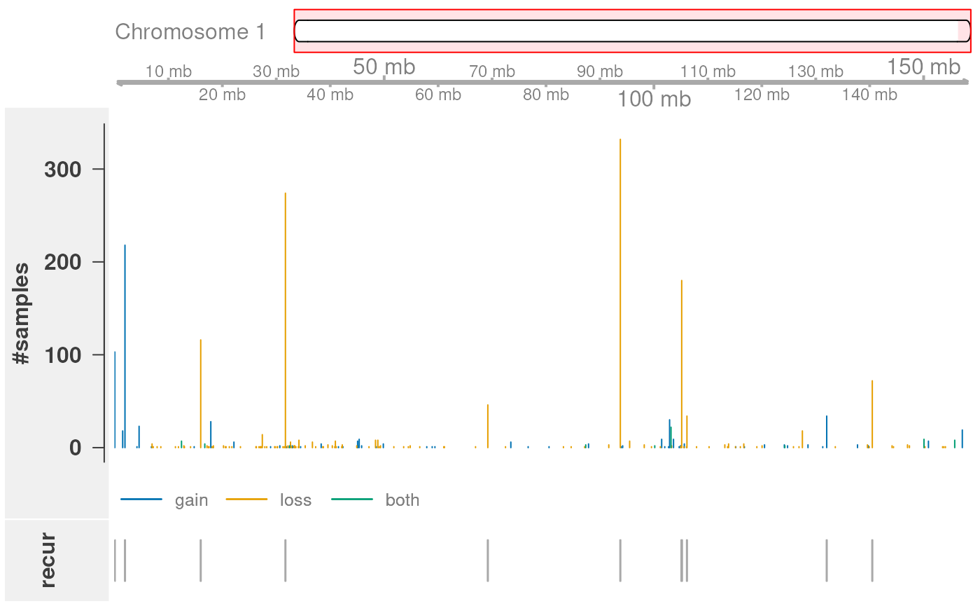
The function plots (from top to bottom): (i) an ideogram of the
chromosome (note that staining bands are not available for
bosTau6), (ii) a genome axis indicating the chromosomal
position, (iii) a bar plot showing for each CNV region the number of
samples with a CNV call in that region, and (iv) an annotation track
that indicates whether this is a recurrent region according to
a significance threshold (an argument to the function, default:
0.05).
Overlap analysis of CNVs with functional genomic regions
 Once individual CNV calls have been summarized across the population, it
is typically of interest whether the resulting CNV regions overlap with
functional genomic regions such as genes, promoters, or enhancers.
Once individual CNV calls have been summarized across the population, it
is typically of interest whether the resulting CNV regions overlap with
functional genomic regions such as genes, promoters, or enhancers.
To obtain the location of protein-coding genes, we query available Bos taurus annotation from Ensembl
library(AnnotationHub)
ah <- AnnotationHub::AnnotationHub()
ahDb <- AnnotationHub::query(ah, pattern = c("Bos taurus", "EnsDb"))
ahDb
## AnnotationHub with 37 records
## # snapshotDate(): 2025-10-29
## # $dataprovider: Ensembl
## # $species: Bos taurus, Bos indicus x Bos taurus
## # $rdataclass: EnsDb
## # additional mcols(): taxonomyid, genome, description,
## # coordinate_1_based, maintainer, rdatadateadded, preparerclass, tags,
## # rdatapath, sourceurl, sourcetype
## # retrieve records with, e.g., 'object[["AH53189"]]'
##
## title
## AH53189 | Ensembl 87 EnsDb for Bos Taurus
## AH53693 | Ensembl 88 EnsDb for Bos Taurus
## AH56658 | Ensembl 89 EnsDb for Bos Taurus
## AH57731 | Ensembl 90 EnsDb for Bos Taurus
## AH60745 | Ensembl 91 EnsDb for Bos Taurus
## ... ...
## AH116763 | Ensembl 112 EnsDb for Bos indicus x Bos taurus
## AH116764 | Ensembl 112 EnsDb for Bos taurus
## AH119223 | Ensembl 113 EnsDb for Bos indicus x Bos taurus
## AH119228 | Ensembl 113 EnsDb for Bos indicus x Bos taurus
## AH119229 | Ensembl 113 EnsDb for Bos taurusand retrieve gene coordinates in the UMD3.1 assembly (Ensembl 92).
ahEdb <- ahDb[["AH60948"]]## loading from cache## require("ensembldb")
bt.genes <- ensembldb::genes(ahEdb)
GenomeInfoDb::seqlevelsStyle(bt.genes) <- "UCSC"
bt.genes
## GRanges object with 24616 ranges and 8 metadata columns:
## seqnames ranges strand | gene_id
## <Rle> <IRanges> <Rle> | <character>
## ENSBTAG00000046619 chr1 19774-19899 - | ENSBTAG00000046619
## ENSBTAG00000006858 chr1 34627-35558 + | ENSBTAG00000006858
## ENSBTAG00000039257 chr1 69695-71121 - | ENSBTAG00000039257
## ENSBTAG00000035349 chr1 83323-84281 - | ENSBTAG00000035349
## ENSBTAG00000001753 chr1 124849-179713 - | ENSBTAG00000001753
## ... ... ... ... . ...
## ENSBTAG00000025951 chrX 148526584-148535857 + | ENSBTAG00000025951
## ENSBTAG00000029592 chrX 148538917-148539037 - | ENSBTAG00000029592
## ENSBTAG00000016989 chrX 148576705-148582356 - | ENSBTAG00000016989
## ENSBTAG00000025952 chrX 148774930-148780901 - | ENSBTAG00000025952
## ENSBTAG00000047839 chrX 148804071-148805135 + | ENSBTAG00000047839
## gene_name gene_biotype seq_coord_system
## <character> <character> <character>
## ENSBTAG00000046619 RF00001 rRNA chromosome
## ENSBTAG00000006858 pseudogene chromosome
## ENSBTAG00000039257 protein_coding chromosome
## ENSBTAG00000035349 pseudogene chromosome
## ENSBTAG00000001753 protein_coding chromosome
## ... ... ... ...
## ENSBTAG00000025951 protein_coding chromosome
## ENSBTAG00000029592 RF00001 rRNA chromosome
## ENSBTAG00000016989 protein_coding chromosome
## ENSBTAG00000025952 protein_coding chromosome
## ENSBTAG00000047839 P2RY8 protein_coding chromosome
## description gene_id_version symbol
## <character> <character> <character>
## ENSBTAG00000046619 NULL ENSBTAG00000046619.1 RF00001
## ENSBTAG00000006858 NULL ENSBTAG00000006858.5
## ENSBTAG00000039257 NULL ENSBTAG00000039257.2
## ENSBTAG00000035349 NULL ENSBTAG00000035349.3
## ENSBTAG00000001753 NULL ENSBTAG00000001753.4
## ... ... ... ...
## ENSBTAG00000025951 NULL ENSBTAG00000025951.4
## ENSBTAG00000029592 NULL ENSBTAG00000029592.1 RF00001
## ENSBTAG00000016989 NULL ENSBTAG00000016989.5
## ENSBTAG00000025952 NULL ENSBTAG00000025952.3
## ENSBTAG00000047839 P2Y receptor family .. ENSBTAG00000047839.1 P2RY8
## entrezid
## <list>
## ENSBTAG00000046619 <NA>
## ENSBTAG00000006858 <NA>
## ENSBTAG00000039257 <NA>
## ENSBTAG00000035349 <NA>
## ENSBTAG00000001753 507243
## ... ...
## ENSBTAG00000025951 <NA>
## ENSBTAG00000029592 <NA>
## ENSBTAG00000016989 <NA>
## ENSBTAG00000025952 785083
## ENSBTAG00000047839 100299937
## -------
## seqinfo: 48 sequences (1 circular) from UMD3.1 genomeTo speed up the example, we restrict analysis to chromosomes 1 and 2.
sel.genes <- subset(bt.genes, seqnames %in% paste0("chr", 1:2))
sel.genes <- subset(sel.genes, gene_biotype == "protein_coding")
sel.cnvrs <- subset(cnvrs, seqnames %in% paste0("chr", 1:2))
Finding and illustrating overlaps
The findOverlaps function from the GenomicRanges
package is a general function for finding overlaps between two sets of
genomic regions. Here, we use the function to find protein-coding genes
(our query region set) overlapping the summarized CNV
regions (our subject region set).
Resulting overlaps are represented as a Hits object,
from which overlapping query and subject regions can be obtained with
dedicated accessor functions (named queryHits and
subjectHits, respectively). Here, we use these functions to
also annotate the CNV type (gain/loss) for genes overlapping with
CNVs.
olaps <- GenomicRanges::findOverlaps(sel.genes, sel.cnvrs, ignore.strand=TRUE)
qh <- S4Vectors::queryHits(olaps)
sh <- S4Vectors::subjectHits(olaps)
cgenes <- sel.genes[qh]
cgenes$type <- sel.cnvrs$type[sh]
subset(cgenes, select = "type")
## GRanges object with 123 ranges and 1 metadata column:
## seqnames ranges strand | type
## <Rle> <IRanges> <Rle> | <character>
## ENSBTAG00000039257 chr1 69695-71121 - | gain
## ENSBTAG00000021819 chr1 1467704-1496151 - | gain
## ENSBTAG00000019404 chr1 1563137-1591758 - | gain
## ENSBTAG00000015212 chr1 1593295-1627137 - | gain
## ENSBTAG00000000597 chr1 18058709-18207251 + | loss
## ... ... ... ... . ...
## ENSBTAG00000003822 chr2 136193743-136239981 - | loss
## ENSBTAG00000013281 chr2 136276529-136314563 + | loss
## ENSBTAG00000009251 chr2 136317925-136337845 - | loss
## ENSBTAG00000008510 chr2 136362255-136444097 + | loss
## ENSBTAG00000014221 chr2 136457565-136461977 + | loss
## -------
## seqinfo: 48 sequences (1 circular) from UMD3.1 genomeIt might also be of interest to illustrate the original CNV calls on
overlapping genomic features (here: protein-coding genes). For this
purpose, an oncoPrint plot provides a useful summary in a
rectangular fashion (genes in the rows, samples in the columns). Stacked
barplots on the top and the right of the plot display the number of
altered genes per sample and the number of altered samples per gene,
respectively.
cnvOncoPrint(grl, cgenes)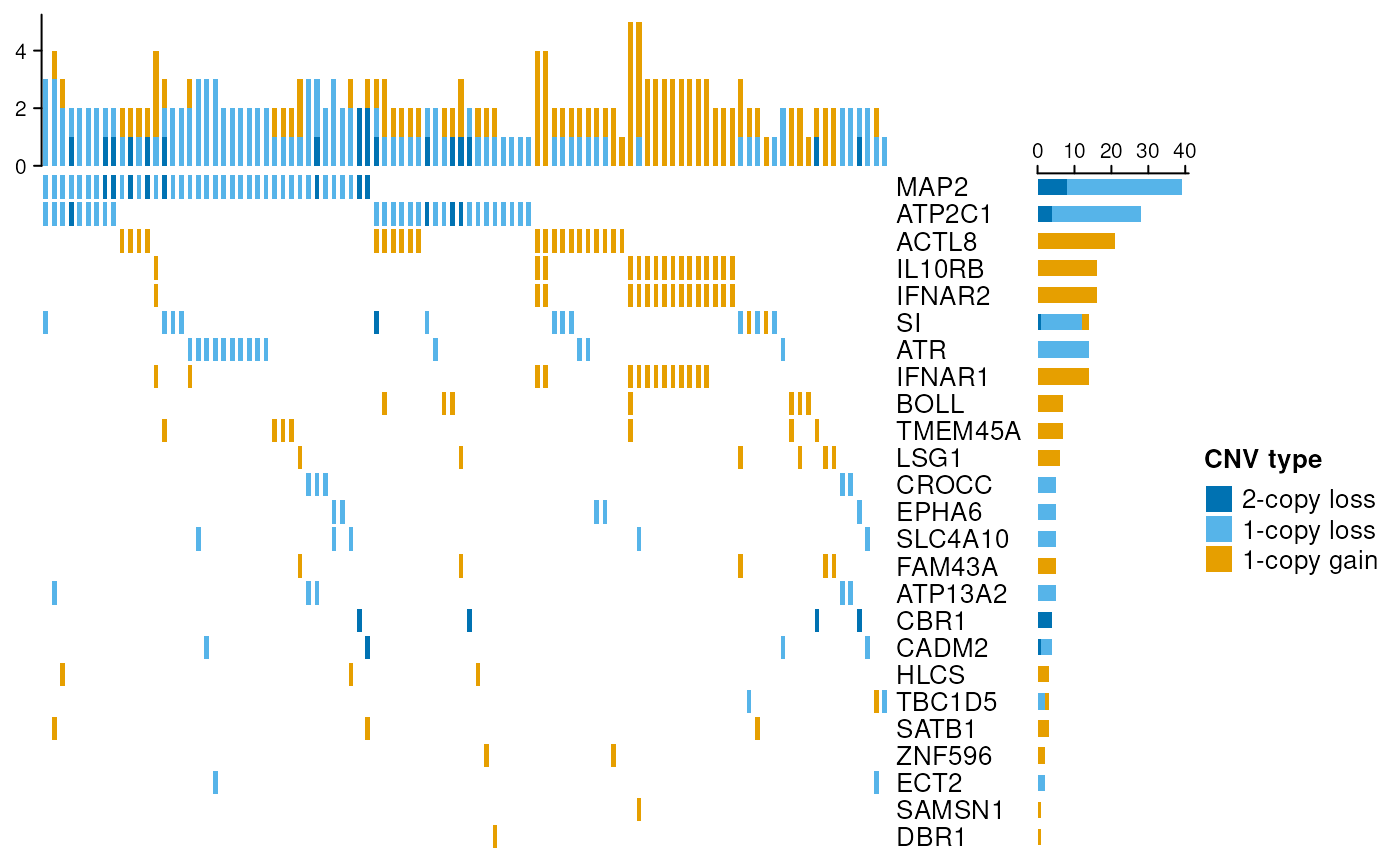
Overlap permutation test
As a certain amount of overlap can be expected just by chance, an assessment of statistical significance is needed to decide whether the observed overlap is greater (enrichment) or less (depletion) than expected by chance.
The regioneR package implements a general framework for testing overlaps of genomic regions based on permutation sampling. This allows to repeatedly sample random regions from the genome, matching size and chromosomal distribution of the region set under study (here: the CNV regions). By recomputing the overlap with the functional features in each permutation, statistical significance of the observed overlap can be assessed.
We demonstrate in the following how this strategy can be used to assess the overlap between the detected CNV regions and protein-coding regions in the cattle genome. We expect to find a depletion as protein-coding regions are highly conserved and rarely subject to long-range structural variation such as CNV. Hence, is the overlap between CNVs and protein-coding genes less than expected by chance?
To answer this question, we apply an overlap permutation test with
100 permutations (ntimes=100), while maintaining
chromosomal distribution of the CNV region set
(per.chromosome=TRUE). Furthermore, we use the option
count.once=TRUE to count an overlapping CNV region only
once, even if it overlaps with 2 or more genes. We also allow random
regions to be sampled from the entire genome (mask=NA),
although in certain scenarios masking certain regions such as telomeres
and centromeres is advisable. Also note that we use 100 permutations for
demonstration only. To draw robust conclusions a minimum of 1000
permutations should be carried out.
library(regioneR)
library(BSgenome.Btaurus.UCSC.bosTau6.masked)
res <- regioneR::overlapPermTest(A=sel.cnvrs, B=sel.genes, ntimes=100,
    genome="bosTau6", mask=NA, per.chromosome=TRUE, count.once=TRUE)
res
## $numOverlaps
## P-value: 0.0099009900990099
## Z-score: -2.3191
## Number of iterations: 100
## Alternative: less
## Evaluation of the original region set: 97
## Evaluation function: numOverlaps
## Randomization function: randomizeRegions
##
## attr(,"class")
## [1] "permTestResultsList"
summary(res[[1]]$permuted)## Min. 1st Qu. Median Mean 3rd Qu. Max.
## 101.0 110.0 115.5 115.7 121.0 137.0The resulting permutation p-value indicates a significant depletion. Out of the 303 CNV regions, 97 overlap with at least one gene. In contrast, when repeatedly drawing random regions matching the CNV regions in size and chromosomal distribution, the mean number of overlapping regions across permutations was 115.7 8.
This finding is consistent with our observations across the whole genome (Silva et al. 2016) and findings from the 1000 Genomes Project (Sudmant et al. 2015).
plot(res)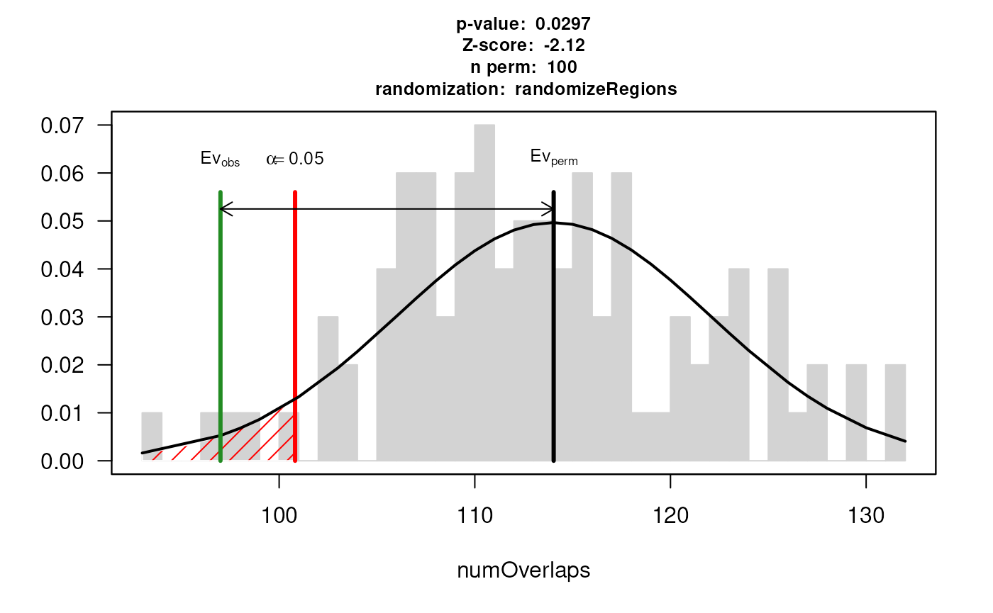
Note: the function regioneR::permTest allows to
incorporate user-defined functions for randomizing regions and
evaluating additional measures of overlap such as total genomic size in
bp.
CNV-expression association analysis
 Studies of expression quantitative trait loci (eQTLs) aim at the
discovery of genetic variants that explain variation in gene expression
levels (Nica and Dermitzakis 2013). Mainly
applied in the context of SNPs, the concept also naturally extends to
the analysis of CNVs.
Studies of expression quantitative trait loci (eQTLs) aim at the
discovery of genetic variants that explain variation in gene expression
levels (Nica and Dermitzakis 2013). Mainly
applied in the context of SNPs, the concept also naturally extends to
the analysis of CNVs.
The CNVRanger package implements association testing between CNV regions and RNA-seq read counts using edgeR, which applies generalized linear models based on the negative-binomial distribution while incorporating normalization factors for different library sizes.
In the case of only one CN state deviating from 2n for a CNV region under investigation, this reduces to the classical 2-group comparison. For more than two states (e.g. 0n, 1n, 2n), edgeR’s ANOVA-like test is applied to test all deviating groups for significant expression differences relative to 2n.
Application to individual CNV and RNA-seq assays
We demonstrate the functionality by loading RNA-seq read count data from skeletal muscle samples for 183 Nelore cattle steers, which we analyzed for CNV-expression effects as previously described (Geistlinger et al. 2018).
rseq.file <- file.path(data.dir, "counts_cleaned.txt")
rcounts <- read.delim(rseq.file, row.names=1, stringsAsFactors=FALSE)
rcounts <- as.matrix(rcounts)
dim(rcounts)
## [1] 939 183
rcounts[1:5, 1:5]## NE001407 NE001408 NE001424 NE001439 NE001448
## ENSBTAG00000000088 64 65 233 135 134
## ENSBTAG00000000160 20 28 50 13 18
## ENSBTAG00000000176 279 373 679 223 417
## ENSBTAG00000000201 252 271 544 155 334
## ENSBTAG00000000210 268 379 486 172 443For demonstration, we restrict analysis to the 939 genes on chromosome 1 and 2, and store the RNA-seq expression data in a SummarizedExperiment.
library(SummarizedExperiment)
rranges <- GenomicRanges::granges(sel.genes)[rownames(rcounts)]
rse <- SummarizedExperiment(assays=list(rcounts=rcounts), rowRanges=rranges)
rse
## class: RangedSummarizedExperiment
## dim: 939 183
## metadata(0):
## assays(1): rcounts
## rownames(939): ENSBTAG00000000088 ENSBTAG00000000160 ...
## ENSBTAG00000048210 ENSBTAG00000048228
## rowData names(0):
## colnames(183): NE001407 NE001408 ... NE003840 NE003843
## colData names(0):Assuming distinct modes of action, effects observed in the CNV-expression analysis are typically divided into (i) local effects (cis), where expression changes coincide with CNVs in the respective genes, and (ii) distal effects (trans), where CNVs supposedly affect trans-acting regulators such as transcription factors.
However, due to power considerations and to avoid detection of spurious effects, stringent filtering of (i) not sufficiently expressed genes, and (ii) CNV regions with insufficient sample size in groups deviating from 2n, should be carried out when testing for distal effects. Local effects have a clear spatial indication and the number of genes locating in or close to a CNV region of interest is typically small; testing for differential expression between CN states is thus generally better powered for local effects and less stringent filter criteria can be applied.
In the following, we carry out CNV-expression association analysis by
providing the CNV regions to test (cnvrs), the individual
CNV calls (grl) to determine per-sample CN state in each
CNV region, the RNA-seq read counts (rse), and the size of
the genomic window around each CNV region (window). The
window argument thereby determines which genes are
considered for testing for each CNV region and is set here to 1 Mbp.
Further, use the filter.by.expr and
min.samples arguments to exclude from the analysis (i)
genes with very low read count across samples, and (ii) CNV regions with
fewer than min.samples samples in a group deviating from
2n.
res <- cnvEQTL(cnvrs, grl, rse, window = "1Mbp", verbose = TRUE)## Restricting analysis to 179 intersecting samples## Preprocessing RNA-seq data ...## Summarizing per-sample CN state in each CNV region## Excluding 286 cnvrs not satisfying min.samples threshold## Analyzing 12 regions with >=1 gene in the given window## 1 of 12## 2 of 12## 3 of 12## 4 of 12## 5 of 12## 6 of 12## 7 of 12## 8 of 12## 9 of 12## 10 of 12## 11 of 12## 12 of 12
res## GRangesList object of length 12:
## $`chr1:16947-111645`
## GRanges object with 5 ranges and 5 metadata columns:
## seqnames ranges strand | logFC.CN0 logFC.CN1
## <Rle> <IRanges> <Rle> | <numeric> <numeric>
## ENSBTAG00000018278 chr1 922635-929992 + | NA NA
## ENSBTAG00000021997 chr1 944294-1188287 - | NA NA
## ENSBTAG00000020035 chr1 351708-362907 + | NA NA
## ENSBTAG00000011528 chr1 463572-478996 - | NA NA
## ENSBTAG00000012594 chr1 669920-733729 - | NA NA
## logFC.CN3 PValue AdjPValue
## <numeric> <numeric> <numeric>
## ENSBTAG00000018278 0.19496712 0.00691099 0.564650
## ENSBTAG00000021997 -0.08125191 0.17695099 0.770648
## ENSBTAG00000020035 0.07451014 0.73843678 0.981503
## ENSBTAG00000011528 0.01209884 0.91331482 0.981503
## ENSBTAG00000012594 -0.00582571 0.94951785 0.981503
## -------
## seqinfo: 48 sequences (1 circular) from UMD3.1 genome
##
## ...
## <11 more elements>The resulting GRangesList contains an entry for each CNV
region tested, storing the genes tested in the genomic window around the
CNV region, and (i) log2 fold change with respect to the 2n group, (ii)
edgeR’s DE p-value, and (iii) the (per default)
Benjamini-Hochberg adjusted p-value.
Application to TCGA data stored in a
MultiAssayExperiment
In the previous section, we individually prepared the CNV and RNA-seq data for CNV-expression association analysis. In the following, we demonstrate how to perform an integrated preparation of the two assays when stored in a MultiAssayExperiment. We therefore consider glioblastoma GBM data from The Cancer Genome Atlas TCGA, which can conveniently be accessed with the curatedTCGAData package.
library(curatedTCGAData)
gbm <- curatedTCGAData::curatedTCGAData("GBM",
        assays=c("GISTIC_Peaks", "CNVSNP", "RNASeq2GeneNorm"),
        version = "1.1.38",
        dry.run=FALSE)
gbm
## A MultiAssayExperiment object of 3 listed
## experiments with user-defined names and respective classes.
## Containing an ExperimentList class object of length 3:
## [1] GBM_CNVSNP-20160128: RaggedExperiment with 146852 rows and 1104 columns
## [2] GBM_GISTIC_Peaks-20160128: RangedSummarizedExperiment with 68 rows and 577 columns
## [3] GBM_RNASeq2GeneNorm-20160128: SummarizedExperiment with 20501 rows and 166 columns
## Functionality:
## experiments() - obtain the ExperimentList instance
## colData() - the primary/phenotype DataFrame
## sampleMap() - the sample coordination DataFrame
## `$`, `[`, `[[` - extract colData columns, subset, or experiment
## *Format() - convert into a long or wide DataFrame
## assays() - convert ExperimentList to a SimpleList of matrices
## exportClass() - save data to flat filesThe returned MultiAssayExperiment contains three
assays:
- the SNP-based CNV calls stored in a
RaggedExperiment(GBM_CNVSNP), - the recurrent CNV regions summarized across the population using the
GISTIC
method (
GBM_GISTIC_Peaks), and - the normalized RNA-seq gene expression values in a
SummarizedExperiment(GBM_RNASeq2GeneNorm).
To annotate the genomic coordinates of the genes measured in the
RNA-seq assay, we use the function symbolsToRanges from the
TCGAutils
package. For demonstration, we restrict the analysis to chromosome 1 and
2.
library(TCGAutils)
gbm <- TCGAutils::symbolsToRanges(gbm, unmapped=FALSE)
## Warning in (function (seqlevels, genome, new_style) : cannot switch some hg19's
## seqlevels from UCSC to NCBI style## Warning: 'experiments' dropped; see 'drops()'
for(i in 1:3)
{
    rr <- rowRanges(gbm[[i]])
    GenomeInfoDb::genome(rr) <- "NCBI37"
    GenomeInfoDb::seqlevelsStyle(rr) <- "UCSC"
    ind <- as.character(seqnames(rr)) %in% c("chr1", "chr2")
    rowRanges(gbm[[i]]) <- rr
    gbm[[i]] <- gbm[[i]][ind,]
}
gbm
## A MultiAssayExperiment object of 3 listed
## experiments with user-defined names and respective classes.
## Containing an ExperimentList class object of length 3:
## [1] GBM_CNVSNP-20160128: RaggedExperiment with 17818 rows and 1104 columns
## [2] GBM_GISTIC_Peaks-20160128: RangedSummarizedExperiment with 12 rows and 577 columns
## [3] GBM_RNASeq2GeneNorm-20160128_ranged: RangedSummarizedExperiment with 2851 rows and 166 columns
## Functionality:
## experiments() - obtain the ExperimentList instance
## colData() - the primary/phenotype DataFrame
## sampleMap() - the sample coordination DataFrame
## `$`, `[`, `[[` - extract colData columns, subset, or experiment
## *Format() - convert into a long or wide DataFrame
## assays() - convert ExperimentList to a SimpleList of matrices
## exportClass() - save data to flat filesWe now restrict the analysis to intersecting patients of the three
assays using MultiAssayExperiment’s
intersectColumns function, and select Primary Solid
Tumor samples using the splitAssays function from the
TCGAutils
package.
gbm <- MultiAssayExperiment::intersectColumns(gbm)
TCGAutils::sampleTables(gbm)
## $`GBM_CNVSNP-20160128`
##
## 01 02 10 11
## 154 13 146 1
##
## $`GBM_GISTIC_Peaks-20160128`
##
## 01
## 154
##
## $`GBM_RNASeq2GeneNorm-20160128_ranged`
##
## 01 02
## 147 13
data(sampleTypes, package="TCGAutils")
sampleTypes
## Code Definition Short.Letter.Code
## 1 01 Primary Solid Tumor TP
## 2 02 Recurrent Solid Tumor TR
## 3 03 Primary Blood Derived Cancer - Peripheral Blood TB
## 4 04 Recurrent Blood Derived Cancer - Bone Marrow TRBM
## 5 05 Additional - New Primary TAP
## 6 06 Metastatic TM
## 7 07 Additional Metastatic TAM
## 8 08 Human Tumor Original Cells THOC
## 9 09 Primary Blood Derived Cancer - Bone Marrow TBM
## 10 10 Blood Derived Normal NB
## 11 11 Solid Tissue Normal NT
## 12 12 Buccal Cell Normal NBC
## 13 13 EBV Immortalized Normal NEBV
## 14 14 Bone Marrow Normal NBM
## 15 15 sample type 15 15SH
## 16 16 sample type 16 16SH
## 17 20 Control Analyte CELLC
## 18 40 Recurrent Blood Derived Cancer - Peripheral Blood TRB
## 19 50 Cell Lines CELL
## 20 60 Primary Xenograft Tissue XP
## 21 61 Cell Line Derived Xenograft Tissue XCL
## 22 99 sample type 99 99SH
gbm <- TCGAutils::TCGAsplitAssays(gbm, sampleCodes="01")
gbm
## A MultiAssayExperiment object of 3 listed
## experiments with user-defined names and respective classes.
## Containing an ExperimentList class object of length 3:
## [1] 01_GBM_CNVSNP-20160128: RaggedExperiment with 17818 rows and 154 columns
## [2] 01_GBM_GISTIC_Peaks-20160128: RangedSummarizedExperiment with 12 rows and 154 columns
## [3] 01_GBM_RNASeq2GeneNorm-20160128_ranged: RangedSummarizedExperiment with 2851 rows and 147 columns
## Functionality:
## experiments() - obtain the ExperimentList instance
## colData() - the primary/phenotype DataFrame
## sampleMap() - the sample coordination DataFrame
## `$`, `[`, `[[` - extract colData columns, subset, or experiment
## *Format() - convert into a long or wide DataFrame
## assays() - convert ExperimentList to a SimpleList of matrices
## exportClass() - save data to flat filesThe SNP-based CNV calls from TCGA are provided as segmented log2 copy number ratios.
## DataFrame with 6 rows and 2 columns
##   Num_Probes Segment_Mean
##    <numeric>    <numeric>
## 1        166       0.1112
## 2          3      -1.2062
## 3      40303       0.1086
## 4        271      -0.3065
## 5      88288       0.1049
## 6      33125       0.3510
summary( mcols(gbm[[ind]])$Segment_Mean )## Min. 1st Qu. Median Mean 3rd Qu. Max.
## -8.2199 -0.9779 -0.0035 -0.6395 0.0493 6.9689It is thus necessary to convert them to integer copy number states for further analysis with CNVRanger.
In a diploid genome, a single-copy gain in a perfectly pure, homogeneous sample has a copy ratio of 3/2. On log2 scale, this is log2(3/2) = 0.585, and a single-copy loss is log2(1/2) = -1.0.
We can roughly convert a log ratio lr to an integer copy
number by
round( (2^lr) * 2)Note that this is not the ideal way to calculate absolute integer copy numbers. Especially in cancer, differences in tumor purity, tumor ploidy, and subclonality can substantially interfere with the assumption of a pure homogeneous sample. See ABSOLUTE (Carter et al. 2012) and the PureCN package for accurately taking such tumor characteristics into account.
However, without additional information we transform the log ratios into integer copy number states using the rough approximation outlined above.
smean <- mcols(gbm[[ind]])$Segment_Mean
state <- round(2^smean * 2)
state[state > 4] <- 4
mcols(gbm[[ind]])$state <- state
gbm[[ind]] <- gbm[[ind]][state != 2,]
mcols(gbm[[ind]]) <- mcols(gbm[[ind]])[,3:1]
table(mcols(gbm[[ind]])$state)
##
## 0 1 3 4
## 2401 4084 1005 747The data is now ready for CNV-expression association analysis, where
we find only four CNV regions with sufficient sample size for testing
using the default value of 10 for the minSamples
argument.
res <- cnvEQTL(cnvrs="01_GBM_GISTIC_Peaks-20160128",
    calls="01_GBM_CNVSNP-20160128",
    rcounts="01_GBM_RNASeq2GeneNorm-20160128_ranged",
    data=gbm, window="1Mbp", verbose=TRUE)
## harmonizing input:
## removing 154 sampleMap rows not in names(experiments)## Preprocessing RNA-seq data ...## Summarizing per-sample CN state in each CNV region## Excluding 4 cnvrs not satisfying min.samples threshold## Analyzing 8 regions with >=1 gene in the given window## 1 of 8## 2 of 8## 3 of 8## 4 of 8## 5 of 8## 6 of 8## 7 of 8## 8 of 8
res## GRangesList object of length 8:
## $`chr1:3394251-6475685`
## GRanges object with 29 ranges and 6 metadata columns:
## seqnames ranges strand | logFC.CN0 logFC.CN1 logFC.CN3
## <Rle> <IRanges> <Rle> | <numeric> <numeric> <numeric>
## RPL22 chr1 6219490-6269449 - | NA -0.658504 -0.0489775
## ICMT chr1 6281253-6296032 - | NA -0.564456 0.4191059
## PHF13 chr1 6673791-6684090 + | NA -0.619955 0.4761981
## KLHL21 chr1 6650784-6674667 - | NA -0.695296 0.3809199
## NOL9 chr1 6581407-6614573 - | NA -0.588524 0.3600387
## ... ... ... ... . ... ... ...
## KCNAB2 chr1 6050987-6161253 + | NA 0.0214685 -0.444799
## TNFRSF14 chr1 2487078-2496821 + | NA 0.0760788 0.294887
## TNFRSF25 chr1 6520846-6526235 - | NA -0.1704237 -0.200658
## TPRG1L chr1 3541579-3546691 + | NA 0.0759256 -0.109257
## PRDM16 chr1 2985732-3355185 + | NA 0.0739074 0.155064
## logFC.CN4 PValue AdjPValue
## <numeric> <numeric> <numeric>
## RPL22 NA 9.69281e-13 8.77738e-12
## ICMT NA 1.16899e-12 1.00287e-11
## PHF13 NA 1.44138e-11 1.17473e-10
## KLHL21 NA 1.33953e-08 9.49320e-08
## NOL9 NA 1.01858e-07 5.76780e-07
## ... ... ... ...
## KCNAB2 NA 0.503633 0.558450
## TNFRSF14 NA 0.518447 0.567160
## TNFRSF25 NA 0.698667 0.734727
## TPRG1L NA 0.722176 0.745030
## PRDM16 NA 0.924857 0.924857
## -------
## seqinfo: 25 sequences (1 circular) from NCBI37 genome
##
## ...
## <7 more elements>We can illustrate differential expression of genes in the
neighborhood of a CNV region of interest using the function
plotEQTL.
res[2]## GRangesList object of length 1:
## $`chr1:7908902-8336254`
## GRanges object with 10 ranges and 6 metadata columns:
## seqnames ranges strand | logFC.CN0 logFC.CN1 logFC.CN3
## <Rle> <IRanges> <Rle> | <numeric> <numeric> <numeric>
## PARK7 chr1 8014351-8045565 + | -2.793668 -0.635210 0.4304657
## SLC45A1 chr1 8378174-8404227 + | -4.120017 -0.651110 0.1860860
## RERE chr1 8412457-8908980 - | -2.211975 -0.728953 0.1688556
## CAMTA1 chr1 6845514-7829766 + | -0.712817 -0.575475 0.1438316
## PER3 chr1 7844351-7905237 + | -2.578312 -0.509463 0.8055643
## ENO1 chr1 8921059-8939249 - | -0.364883 -0.450647 0.5066135
## VAMP3 chr1 7831356-7841492 + | -0.951620 -0.394923 0.1872536
## ERRFI1 chr1 8064464-8086369 - | -3.587187 -0.403047 -0.1225251
## H6PD chr1 9294833-9331396 + | -1.166641 -0.374257 0.1458584
## SLC2A5 chr1 9095165-9148537 - | -0.625280 -0.275883 -0.0746078
## logFC.CN4 PValue AdjPValue
## <numeric> <numeric> <numeric>
## PARK7 NA 1.32063e-17 1.79386e-16
## SLC45A1 NA 3.52005e-15 3.82512e-14
## RERE NA 2.82806e-13 2.71161e-12
## CAMTA1 NA 2.60588e-08 1.69904e-07
## PER3 NA 1.93529e-05 8.08850e-05
## ENO1 NA 1.25499e-04 4.44704e-04
## VAMP3 NA 1.46285e-04 4.96758e-04
## ERRFI1 NA 4.07423e-04 1.27711e-03
## H6PD NA 1.08233e-02 2.10024e-02
## SLC2A5 NA 5.11493e-01 5.63333e-01
## -------
## seqinfo: 25 sequences (1 circular) from NCBI37 genome## GRanges object with 1 range and 0 metadata columns:
## seqnames ranges strand
## <Rle> <IRanges> <Rle>
## [1] chr1 7908902-8336254 *
## -------
## seqinfo: 1 sequence from an unspecified genome; no seqlengths
plotEQTL(cnvr=r, genes=res[[2]], genome="hg19", cn="CN1")
The plot shows consistent decreased expression (negative log2 fold change) of genes in the neighborhood of the CNV region, when comparing samples with a one copy loss (1) in that region to the 2 reference group.
Note that a significant expression change is not only observed for genes locating within the CNV region (dosage effect, here: PARK7), but also genes locating in close proximity of the CNV region (neighborhood effect, here: CAMTA1 and RERE). This is consistent with previous observations in mouse (Cahan et al. 2009) and our observations in cattle (Geistlinger et al. 2018).
CNV-phenotype association analysis
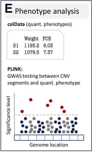 Specifically developed for CNV calls inferred from SNP-chip data, CNVRanger
allows to carry out a probe-level genome-wide association study (GWAS)
with quantitative phenotypes. CNV calls from other sources such as
sequencing data are also supported by using the start and end position
of each call as the corresponding probes.
Specifically developed for CNV calls inferred from SNP-chip data, CNVRanger
allows to carry out a probe-level genome-wide association study (GWAS)
with quantitative phenotypes. CNV calls from other sources such as
sequencing data are also supported by using the start and end position
of each call as the corresponding probes.
As previously described (Silva et al.
2016), we construct CNV segments from probes representing common
CN polymorphisms (allele frequency >1%), and carry out a GWAS using a
standard linear regression of phenotype on allele dosage with the
lm function.
For CNV segments composed of multiple probes, the segment p-value is chosen from the probe p-values, using either the probe with minimum p-value or the probe with maximum CNV frequency.
For demonstration, we use CNV data of a wild population of songbirds (Silva et al. 2018).
cnv.loc <- file.path(data.dir, "CNVOut.txt")
cnv.calls <- read.delim(cnv.loc, as.is=TRUE)
head(cnv.calls)
## chr start end sample.id state num.snps start.probe end.probe
## 1 25 6463188 6475943 1068 3 12 AX-100224358 AX-100363929
## 2 1 98166149 98184039 1068 3 28 AX-100796878 AX-100422118
## 3 4 67895958 67938901 1068 3 8 AX-100222654 AX-100726215
## 4 8 30702029 30722351 1334 3 13 AX-100160546 AX-100828216
## 5 2 877347 942971 1334 3 26 AX-100292215 AX-100391883
## 6 1 98147555 98186543 546 3 48 AX-100939600 AX-100309013Here, we use the extensibility of the basic five-column input format described in Section 4.1. In addition to the required five columns (providing chromosome, start position, end position, sample ID, and integer copy number state), we provided three optional columns storing the number of probes supporting the call, and the Affymetrix ID of the first and last probe contained in the call.
As these columns are optional, it is not ultimately necessary to provide them in order to run a CNV GWAS. However, we recommend to provide this information when available as it allows for a more fine-grained probe-by-probe GWAS.
As described in Section
4.2, we store the CNV calls in a GRangesList for
further analysis.
cnv.calls <- GenomicRanges::makeGRangesListFromDataFrame(cnv.calls,
    split.field="sample.id", keep.extra.columns=TRUE)
sort(cnv.calls)
## GRangesList object of length 10:
## $`112`
## GRanges object with 2 ranges and 4 metadata columns:
## seqnames ranges strand | state num.snps start.probe
## <Rle> <IRanges> <Rle> | <integer> <integer> <character>
## [1] 1 100727703-100730748 * | 0 8 AX-100388724
## [2] 10 19062731-19096193 * | 3 9 AX-100271359
## end.probe
## <character>
## [1] AX-100765659
## [2] AX-100147230
## -------
## seqinfo: 10 sequences from an unspecified genome; no seqlengths
##
## $`175`
## GRanges object with 2 ranges and 4 metadata columns:
## seqnames ranges strand | state num.snps start.probe
## <Rle> <IRanges> <Rle> | <integer> <integer> <character>
## [1] 8 4122253-4193189 * | 3 62 AX-100097083
## [2] 27 2299391-2308228 * | 3 6 AX-100610990
## end.probe
## <character>
## [1] AX-100912769
## [2] AX-100178489
## -------
## seqinfo: 10 sequences from an unspecified genome; no seqlengths
##
## $`356`
## GRanges object with 1 range and 4 metadata columns:
## seqnames ranges strand | state num.snps start.probe
## <Rle> <IRanges> <Rle> | <integer> <integer> <character>
## [1] 1 100728444-100730748 * | 0 6 AX-100700982
## end.probe
## <character>
## [1] AX-100765659
## -------
## seqinfo: 10 sequences from an unspecified genome; no seqlengths
##
## ...
## <7 more elements>In the following, we use genomic estimated breeding values (GEBVs) for breeding time (BT) as the quantitative phenotype, and accordingly analyze for each CNV region whether change in copy number is associated with change in the genetic potential for breeding time.
Setting up a CNV-GWAS
We read phenotype information from a tab-delimited file, containing exactly four columns: sample ID, family ID, sex, and the quantitative phenotype (here: breeding time, BT) because we use the PLINK input format for compatibility.
phen.loc <- file.path(data.dir, "Pheno.txt")
colData <- read.delim(phen.loc, as.is=TRUE)
head(colData)
## sample.id fam sex BT
## 1 911 NA 2 -2.842842
## 2 622 NA 2 -2.884186
## 3 1195 622 2 -3.062731
## 4 112 NA 2 -3.161435
## 5 175 NA 2 -3.597768
## 6 2391 NA 2 3.623262Although fam and sex are listed as columns,
this info is not considered in the current implementation and can be set
to NA.
As described in Section 4.3, we combine
the CNV calls with the phenotype information in a
RaggedExperiment for coordinated representation and
analysis.
mcols(cnv.calls) <- colData
re <- RaggedExperiment::RaggedExperiment(cnv.calls)
re
## class: RaggedExperiment
## dim: 19 10
## assays(4): state num.snps start.probe end.probe
## rownames: NULL
## colnames(10): 112 175 ... 1334 2391
## colData names(4): sample.id fam sex BTIf probe information is available and has been annotated to the CNV calls, as we did above, the probe IDs and corresponding genomic positions should be provided in a separate file.
Map file is expected to be a tab-delimited file containing exactly three columns: probe ID,chromosome, and the position in bp. Map file is optional. If no map file is provided a pseudomap will be automatically generated.
map.loc <- file.path(data.dir, "MapPenn.txt")
map.df <- read.delim(map.loc, as.is=TRUE)
head(map.df)
## Name Chr Position
## 1 AX-100939600 1 98147555
## 2 AX-100088448 1 98148072
## 3 AX-100954037 1 98150537
## 4 AX-100836117 1 98151270
## 5 AX-100027637 1 98151959
## 6 AX-100215062 1 98151992Given a RaggedExperiment storing CNV calls together with
phenotype information, and optionally a map file for probe-level
coordinates, the setupCnvGWAS function sets up all files
needed for the GWAS analysis.
The information required for analysis is stored in the resulting
phen.info list:
phen.info <- setupCnvGWAS("example", cnv.out.loc=re, map.loc=map.loc)
phen.info
## $samplesPhen
## [1] "911" "622" "1195" "112" "175" "2391" "1068" "546" "356" "1334"
##
## $phenotypes
## [1] "BT"
##
## $phenotypesdf
## BT
## 1 -2.842842
## 2 -2.884186
## 3 -3.062731
## 4 -3.161435
## 5 -3.597768
## 6 3.623262
## 7 3.216123
## 8 3.129881
## 9 3.106459
## 10 3.004740
##
## $phenotypesSam
## samplesPhen BT
## 1 911 -2.842842
## 2 622 -2.884186
## 3 1195 -3.062731
## 4 112 -3.161435
## 5 175 -3.597768
## 6 2391 3.623262
## 7 1068 3.216123
## 8 546 3.129881
## 9 356 3.106459
## 10 1334 3.004740
##
## $FamID
## samplesPhen V2
## 1 911 NA
## 2 622 NA
## 3 1195 622
## 4 112 NA
## 5 175 NA
## 6 2391 NA
## 7 1068 NA
## 8 546 NA
## 9 356 NA
## 10 1334 NA
##
## $SexIds
## samplesPhen V2
## 1 911 2
## 2 622 2
## 3 1195 2
## 4 112 2
## 5 175 2
## 6 2391 2
## 7 1068 2
## 8 546 2
## 9 356 2
## 10 1334 2
##
## $all.paths
## Inputs
## "~/.local/share/CNVRanger/example/Inputs"
## Results
## "~/.local/share/CNVRanger/example/Results"The last item of the list displays the working directory:
all.paths <- phen.info$all.paths
all.paths
## Inputs
## "~/.local/share/CNVRanger/example/Inputs"
## Results
## "~/.local/share/CNVRanger/example/Results"For the GWAS, chromosome names are assumed to be integer
(i.e. 1, 2, 3, ...). Non-integer chromosome names can be
encoded by providing a data.frame that describes the
mapping from character names to corresponding integers.
For the example data, chromosomes 1A, 4A, 25LG1, 25LG2, and LGE22 are correspondingly encoded via
# Define chr correspondence to numeric
chr.code.name <- data.frame(
                    V1 = c(16, 25, 29:31),
                    V2 = c("1A", "4A", "25LG1", "25LG2", "LGE22"))
Running a CNV-GWAS
We can then run the actual CNV-GWAS, here without correction for multiple testing which is done for demonstration only. In real analyses, multiple testing correction is recommended to avoid inflation of false positive findings.
segs.pvalue.gr <- cnvGWAS(phen.info, chr.code.name=chr.code.name, method.m.test="none")
segs.pvalue.gr
## GRanges object with 16 ranges and 6 metadata columns:
## seqnames ranges strand | SegName MinPvalue NameProbe
## <Rle> <IRanges> <Rle> | <integer> <numeric> <character>
## [1] 1 98171563-98184039 * | 2 0.0323047 AX-100337994
## [2] 8 4121283-4188293 * | 7 0.0349439 AX-100097083
## [3] 8 4193189 * | 8 0.1124385 AX-100912769
## [4] 1 98186123-98186543 * | 3 0.1201779 AX-100364577
## [5] 1 98147555-98171009 * | 1 0.1976503 AX-100195917
## ... ... ... ... . ... ... ...
## [12] 18 1278467-1295371 * | 13 0.385570 AX-100573546
## [13] 11 18840662 * | 12 0.392639 AX-100673859
## [14] 21 3326720-3329134 * | 14 0.392639 AX-100389358
## [15] 11 18836038-18839377 * | 11 0.968849 AX-100780252
## [16] 1 100728444-100730326 * | 4 0.972202 AX-100700982
## Frequency MinPvalueAdjusted Phenotype
## <character> <numeric> <character>
## [1] 3 0.03230 BT
## [2] 3 0.03494 BT
## [3] 2 0.11244 BT
## [4] 2 0.12018 BT
## [5] 4 0.19765 BT
## ... ... ... ...
## [12] 1 0.38557 BT
## [13] 1 0.39264 BT
## [14] 1 0.39264 BT
## [15] 2 0.96885 BT
## [16] 2 0.97220 BT
## -------
## seqinfo: 10 sequences from an unspecified genome; no seqlengthsThe CNV-GWAS uses the concept of CNV segments to define more fine-grained CNV loci within CNV regions.
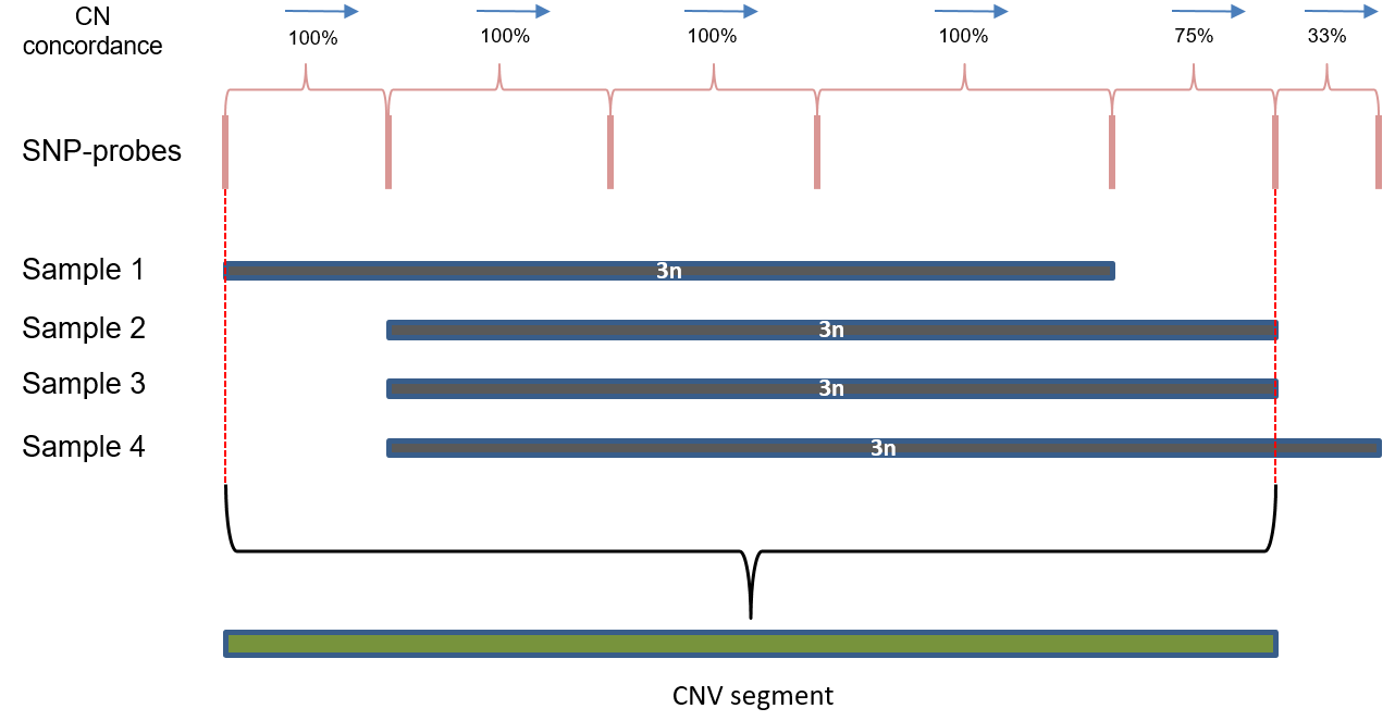
Definition of CNV segments. The figure shows construction of a CNV segment from 4 individual CNV calls in a CNV region based on pairwise copy number concordance between adjacent probes.
This procedure was originally proposed in our previous work in Nelore cattle (Silva et al. 2016) and defines CNV segments based on CNV genotype similarity of subsequent SNP probes.
The default is min.sim=0.95, which will continuously add
probe positions to a given CNV segment until the pairwise genotype
similarity drops below 95%. An example of detailed up-down CNV genotype
concordance that is used for the construction of CNV segments is given
in S12 Table in (Silva et al. 2016).
Only one of the p-values of the probes contained in a CNV segment is chosen as the segment p-value. This is similar to a common approach used in differential expression (DE) analysis of microarray gene expression data, where typically the most significant DE probe is chosen in case of multiple probes mapping to the same gene.
Here, the representative probe for the CNV segment can be chosen to
be the probe with lowest p-value
(assign.probe="min.pvalue", default) or the one with
highest CNV frequency (assign.probe="high.freq").
Multiple testing correction based on the number of CNV segments tested is carried out using the FDR approach (default). Results can then be displayed as for regular GWAS via a Manhattan plot (which can optionally be exported to a pdf file).
## Define the chromosome order in the plot
order.chrs <- c(1:24, "25LG1", "25LG2", 27:28, "LGE22", "1A", "4A")

## Chromosome sizes
chr.size.file <- file.path(data.dir, "Parus_major_chr_sizes.txt")
chr.sizes <- scan(chr.size.file)
chr.size.order <- data.frame(chr=order.chrs, sizes=chr.sizes, stringsAsFactors=FALSE)

## Plot a pdf file with a manhatthan within the 'Results' workfolder
plotManhattan(all.paths, segs.pvalue.gr, chr.size.order, plot.pdf=FALSE)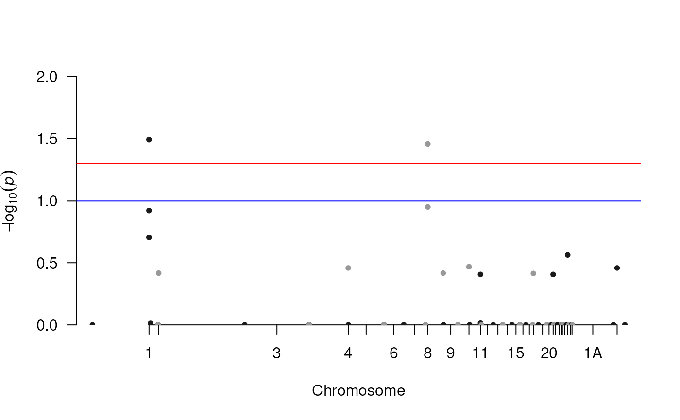
Producing a GDS file in advance
The genomic data structure (GDS) file format supports efficient
memory management for genotype analysis. To make use of this efficient
data representation, CNV genotypes analyzed with the
cnvGWAS function are stored in a CNV.gds file,
which is automatically produced and placed in the Inputs
folder (i.e. all.paths[1]).
Therefore, running a GWAS implies that any GDS file produced by
previous analysis will be overwritten. Use
produce.gds=FALSE to avoid overwriting in the GWAS run.
For convenience, a GDS file can be produced before the GWAS analysis
with the generateGDS function. This additionally returns a
GRanges object containing the genomic position, name and,
frequency of each probe used to construct the CNV segments for the GWAS
analysis.
Note that probes.cnv.gr object contains the integer
chromosome names (as the GDS file on disk). Only the
segs.pvalue.gr, which stores the GWAS results, has the
character chromosome names.
## Create a GDS file in disk and export the SNP probe positions
probes.cnv.gr <- generateGDS(phen.info, chr.code.name=chr.code.name)
probes.cnv.gr
## GRanges object with 189 ranges and 3 metadata columns:
## seqnames ranges strand | Name freq snp.id
## <Rle> <IRanges> <Rle> | <character> <integer> <integer>
## [1] 1 98147555 * | AX-100939600 2 1
## [2] 1 98148072 * | AX-100088448 2 2
## [3] 1 98150537 * | AX-100954037 2 3
## [4] 1 98151270 * | AX-100836117 2 4
## [5] 1 98151959 * | AX-100027637 2 5
## ... ... ... ... . ... ... ...
## [185] 25 6471766 * | AX-100066308 1 185
## [186] 25 6473449 * | AX-100023435 1 186
## [187] 25 6474550 * | AX-100397956 1 187
## [188] 25 6475943 * | AX-100363929 1 188
## [189] 27 2308228 * | AX-100178489 1 189
## -------
## seqinfo: 15 sequences from an unspecified genome; no seqlengths
## Run GWAS with existent GDS file
segs.pvalue.gr <- cnvGWAS(phen.info, chr.code.name=chr.code.name, produce.gds=FALSE)
Using relative signal intensities
SNP-based CNV callers such as PennCNV and Birdsuit infer CNVs from SNP-chip intensities (log R ratios, LRRs) and allele frequencies (B allelel frequencies, BAFs). As an auxiliary analysis, it can be interesting to carry out the GWAS based on the LRR relative signal intensities itself (Silva et al. 2018).
To perform the GWAS using LRR values, import the LRR/BAF values and
set run.lrr=TRUE in the cnvGWAS function:
# List files to import LRR/BAF
files <- list.files(data.dir, pattern = "\\.cnv.txt.adjusted$")
samples <- sub(".cnv.txt.adjusted$", "", files)
samples <- sub("^GT","", samples)
sample.files <- data.frame(file.names=files, sample.names=samples)

# All missing samples will have LRR = '0' and BAF = '0.5' in all SNPs listed in the GDS file
importLrrBaf(all.paths, data.dir, sample.files, verbose=FALSE)

# Read the GDS to check if the LRR/BAF nodes were added
cnv.gds <- file.path(all.paths[1], "CNV.gds")
(genofile <- SNPRelate::snpgdsOpen(cnv.gds, allow.fork=TRUE, readonly=FALSE))
## File: /github/home/.local/share/CNVRanger/example/Inputs/CNV.gds (49.7K)
## + [ ] *
## |--+ sample.id { Str8 10 ZIP_ra(122.7%), 61B }
## |--+ snp.id { Str8 189 ZIP_ra(45.4%), 301B }
## |--+ snp.rs.id { Str8 189 ZIP_ra(31.9%), 791B }
## |--+ snp.position { Int32 189 ZIP_ra(86.2%), 659B }
## |--+ snp.chromosome { Str8 189 ZIP_ra(11.8%), 56B }
## |--+ genotype { Bit2 189x10, 473B } *
## |--+ CNVgenotype { Float64 189x10, 14.8K }
## |--+ phenotype [ data.frame ] *
## | |--+ samplesPhen { Str8 10, 44B }
## | \--+ BT { Float64 10, 80B }
## |--+ FamID { Str8 10, 13B }
## |--+ Sex { Str8 10, 20B }
## |--+ Chr.names [ data.frame ] *
## | |--+ V1 { Float64 5, 40B }
## | \--+ V2 { Str8 5, 24B }
## |--+ LRR { Float64 189x10, 14.8K }
## \--+ BAF { Float64 189x10, 14.8K }
gdsfmt::closefn.gds(genofile)

# Run the CNV-GWAS with existent GDS
segs.pvalue.gr <- cnvGWAS(phen.info, chr.code.name=chr.code.name, produce.gds=FALSE, run.lrr=TRUE)
Session info
## R version 4.5.2 (2025-10-31)
## Platform: x86_64-pc-linux-gnu
## Running under: Ubuntu 24.04.3 LTS
##
## Matrix products: default
## BLAS:   /usr/lib/x86_64-linux-gnu/openblas-pthread/libblas.so.3
## LAPACK: /usr/lib/x86_64-linux-gnu/openblas-pthread/libopenblasp-r0.3.26.so;  LAPACK version 3.12.0
##
## locale:
##  [1] LC_CTYPE=en_US.UTF-8       LC_NUMERIC=C
##  [3] LC_TIME=en_US.UTF-8        LC_COLLATE=en_US.UTF-8
##  [5] LC_MONETARY=en_US.UTF-8    LC_MESSAGES=en_US.UTF-8
##  [7] LC_PAPER=en_US.UTF-8       LC_NAME=C
##  [9] LC_ADDRESS=C               LC_TELEPHONE=C
## [11] LC_MEASUREMENT=en_US.UTF-8 LC_IDENTIFICATION=C
##
## time zone: Etc/UTC
## tzcode source: system (glibc)
##
## attached base packages:
## [1] grid      stats4    stats     graphics  grDevices utils     datasets
## [8] methods   base
##
## other attached packages:
##  [1] ensembldb_2.34.0
##  [2] AnnotationFilter_1.34.0
##  [3] GenomicFeatures_1.62.0
##  [4] AnnotationDbi_1.72.0
##  [5] Gviz_1.54.0
##  [6] TCGAutils_1.29.5
##  [7] curatedTCGAData_1.32.0
##  [8] MultiAssayExperiment_1.36.0
##  [9] SummarizedExperiment_1.40.0
## [10] Biobase_2.70.0
## [11] MatrixGenerics_1.22.0
## [12] matrixStats_1.5.0
## [13] BSgenome.Btaurus.UCSC.bosTau6.masked_1.3.99
## [14] BSgenome.Btaurus.UCSC.bosTau6_1.4.0
## [15] BSgenome_1.78.0
## [16] rtracklayer_1.70.0
## [17] BiocIO_1.20.0
## [18] Biostrings_2.78.0
## [19] XVector_0.50.0
## [20] regioneR_1.42.0
## [21] AnnotationHub_4.0.0
## [22] BiocFileCache_3.0.0
## [23] dbplyr_2.5.1
## [24] CNVRanger_1.26.0
## [25] RaggedExperiment_1.34.0
## [26] GenomicRanges_1.62.0
## [27] Seqinfo_1.0.0
## [28] IRanges_2.44.0
## [29] S4Vectors_0.48.0
## [30] BiocGenerics_0.56.0
## [31] generics_0.1.4
## [32] BiocStyle_2.38.0
##
## loaded via a namespace (and not attached):
##   [1] splines_4.5.2
##   [2] bitops_1.0-9
##   [3] filelock_1.0.3
##   [4] tibble_3.3.0
##   [5] XML_3.99-0.20
##   [6] rpart_4.1.24
##   [7] lifecycle_1.0.4
##   [8] httr2_1.2.1
##   [9] edgeR_4.8.0
##  [10] doParallel_1.0.17
##  [11] MASS_7.3-65
##  [12] lattice_0.22-7
##  [13] backports_1.5.0
##  [14] magrittr_2.0.4
##  [15] limma_3.66.0
##  [16] Hmisc_5.2-4
##  [17] sass_0.4.10
##  [18] rmarkdown_2.30
##  [19] jquerylib_0.1.4
##  [20] yaml_2.3.10
##  [21] DBI_1.2.3
##  [22] RColorBrewer_1.1-3
##  [23] abind_1.4-8
##  [24] rvest_1.0.5
##  [25] purrr_1.2.0
##  [26] gdsfmt_1.46.0
##  [27] biovizBase_1.58.0
##  [28] RCurl_1.98-1.17
##  [29] nnet_7.3-20
##  [30] VariantAnnotation_1.56.0
##  [31] rappdirs_0.3.3
##  [32] circlize_0.4.16
##  [33] pkgdown_2.2.0
##  [34] codetools_0.2-20
##  [35] DelayedArray_0.36.0
##  [36] xml2_1.4.1
##  [37] tidyselect_1.2.1
##  [38] shape_1.4.6.1
##  [39] UCSC.utils_1.6.0
##  [40] farver_2.1.2
##  [41] base64enc_0.1-3
##  [42] GenomicAlignments_1.46.0
##  [43] jsonlite_2.0.0
##  [44] GetoptLong_1.0.5
##  [45] Formula_1.2-5
##  [46] iterators_1.0.14
##  [47] systemfonts_1.3.1
##  [48] foreach_1.5.2
##  [49] tools_4.5.2
##  [50] progress_1.2.3
##  [51] TxDb.Hsapiens.UCSC.hg19.knownGene_3.22.1
##  [52] ragg_1.5.0
##  [53] SNPRelate_1.44.0
##  [54] Rcpp_1.1.0
##  [55] glue_1.8.0
##  [56] GenomicDataCommons_1.34.1
##  [57] gridExtra_2.3
##  [58] SparseArray_1.10.1
##  [59] BiocBaseUtils_1.12.0
##  [60] xfun_0.54
##  [61] GenomeInfoDb_1.46.0
##  [62] dplyr_1.1.4
##  [63] withr_3.0.2
##  [64] BiocManager_1.30.27
##  [65] fastmap_1.2.0
##  [66] latticeExtra_0.6-31
##  [67] digest_0.6.38
##  [68] R6_2.6.1
##  [69] textshaping_1.0.4
##  [70] colorspace_2.1-2
##  [71] jpeg_0.1-11
##  [72] dichromat_2.0-0.1
##  [73] biomaRt_2.66.0
##  [74] RSQLite_2.4.4
##  [75] cigarillo_1.0.0
##  [76] RhpcBLASctl_0.23-42
##  [77] calibrate_1.7.7
##  [78] data.table_1.17.8
##  [79] prettyunits_1.2.0
##  [80] httr_1.4.7
##  [81] htmlwidgets_1.6.4
##  [82] S4Arrays_1.10.0
##  [83] pkgconfig_2.0.3
##  [84] gtable_0.3.6
##  [85] blob_1.2.4
##  [86] ComplexHeatmap_2.26.0
##  [87] S7_0.2.1
##  [88] htmltools_0.5.8.1
##  [89] bookdown_0.45
##  [90] ProtGenerics_1.42.0
##  [91] clue_0.3-66
##  [92] scales_1.4.0
##  [93] png_0.1-8
##  [94] knitr_1.50
##  [95] rstudioapi_0.17.1
##  [96] tzdb_0.5.0
##  [97] rjson_0.2.23
##  [98] checkmate_2.3.3
##  [99] curl_7.0.0
## [100] org.Hs.eg.db_3.22.0
## [101] cachem_1.1.0
## [102] GlobalOptions_0.1.2
## [103] stringr_1.6.0
## [104] BiocVersion_3.22.0
## [105] parallel_4.5.2
## [106] foreign_0.8-90
## [107] restfulr_0.0.16
## [108] desc_1.4.3
## [109] pillar_1.11.1
## [110] vctrs_0.6.5
## [111] cluster_2.1.8.1
## [112] htmlTable_2.4.3
## [113] qqman_0.1.9
## [114] evaluate_1.0.5
## [115] readr_2.1.6
## [116] locfit_1.5-9.12
## [117] cli_3.6.5
## [118] compiler_4.5.2
## [119] Rsamtools_2.26.0
## [120] rlang_1.1.6
## [121] crayon_1.5.3
## [122] interp_1.1-6
## [123] plyr_1.8.9
## [124] fs_1.6.6
## [125] stringi_1.8.7
## [126] deldir_2.0-4
## [127] BiocParallel_1.44.0
## [128] lazyeval_0.2.2
## [129] Matrix_1.7-4
## [130] ExperimentHub_3.0.0
## [131] hms_1.1.4
## [132] bit64_4.6.0-1
## [133] ggplot2_4.0.1
## [134] statmod_1.5.1
## [135] KEGGREST_1.50.0
## [136] memoise_2.0.1
## [137] bslib_0.9.0
## [138] bit_4.6.0