Focused Sub-Analysis of Breast Cancer Microbial Signatures

Introduction

This vignette demonstrates a focused sub-analysis of microbial signatures associated specifically with breast cancer using BugSigDB. Unlike the Cervical Cancer sub-analysis, no body-site restriction is applied by default here: breast cancer microbiome research spans both breast tissue itself and fecal/gut samples (investigating the gut-breast axis), so restricting to breast tissue alone would discard a substantial, legitimately relevant portion of the evidence base. This notebook also evaluates how breast-cancer-associated taxa overlap with other broader women’s health conditions.

Download and Prepare Data

full.dat <- bugsigdbr::importBugSigDB(cache = FALSE)

# Remove empty signatures
ind1 <- lengths(full.dat[["MetaPhlAn taxon names"]]) > 0
ind2 <- lengths(full.dat[["NCBI Taxonomy IDs"]]) > 0
dat <- full.dat[ind1 & ind2, ]

Select Breast Cancer Specific Signatures

breast_terms <- c(
  "Breast cancer",
  "Breast cancer stage",
  "Breast carcinoma",
  "HER2 Positive Breast Carcinoma"
)

breast_dat <- dat %>%
  filter(Condition %in% breast_terms) %>%
  distinct()

nrow(breast_dat)

## [1] 43

breast_dat %>%
  count(Condition, sort = TRUE) %>%
  knitr::kable()

Condition	n
Breast cancer	33
Breast carcinoma	6
Breast cancer stage	2
HER2 Positive Breast Carcinoma	2

Study Characteristics

study.summary <- breast_dat %>%
  count(`Body site`, `Sequencing type`)

knitr::kable(study.summary)

Body site	Sequencing type	n
Breast	16S	8
Feces	16S	22
Feces	WMS	9
Feces,Saliva	16S	2
Saliva	16S	2

breast_dat %>%
  count(Year) %>%
  arrange(Year) %>%
  knitr::kable()

Year	n
2017	2
2018	2
2020	6
2021	8
2022	6
2023	4
2024	15

The body site breakdown above shows how the evidence splits between breast tissue itself and other sites (most likely feces, reflecting gut-breast axis research). Review this table before deciding whether a body-site restriction is warranted for your specific research question - the default here keeps all sites.

Demographic & Anatomy Metrics Visualisations

breast_dat %>%
  count(`Body site`, sort = TRUE) %>%
  ggplot(aes(x = reorder(`Body site`, n), y = n)) +
  geom_col(fill = "#C71585", width = 0.6) +
  coord_flip() +
  labs(
    title = "Breast Cancer Signatures by Body Site",
    subtitle = "Distribution of tissue sampling locations across studies",
    x = NULL, y = "Number of Signatures"
  ) +
  theme_minimal(base_size = 11) +
  theme(plot.title = element_text(face = "bold"))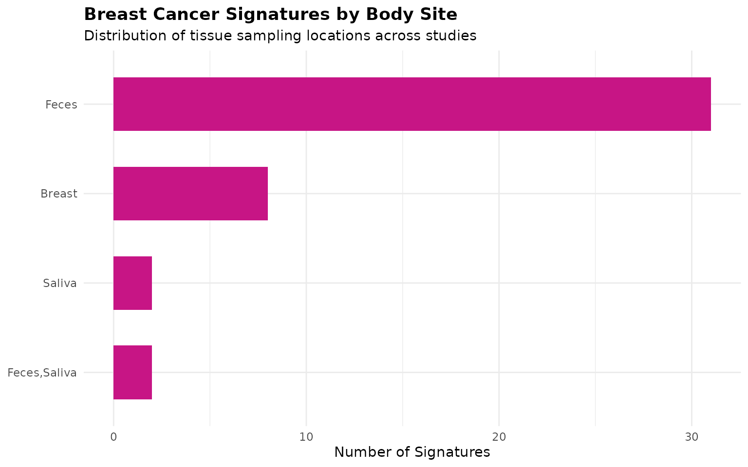

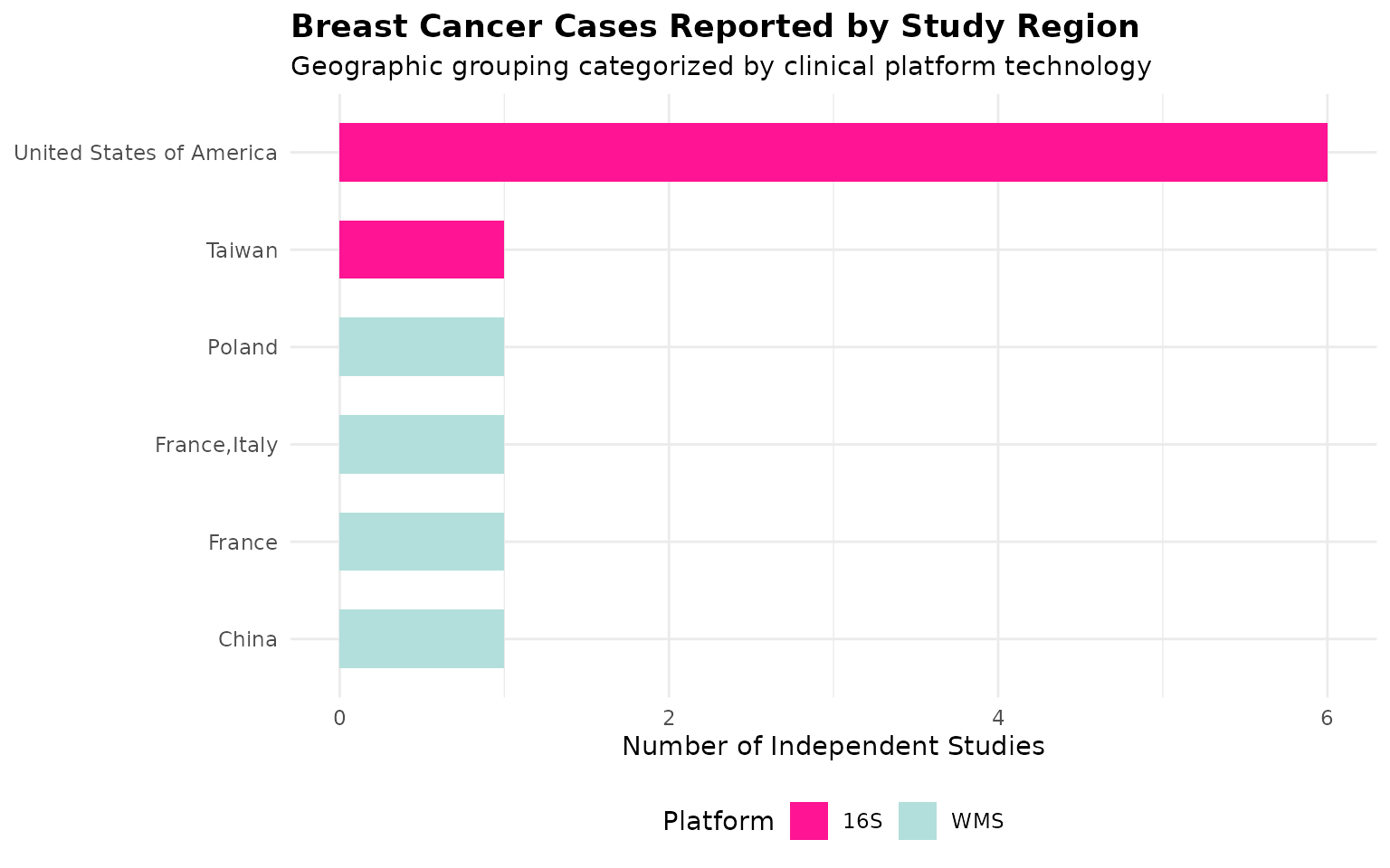
breast_dat %>%
  distinct(PMID, `Location of subjects`, `Sequencing type`) %>%
  count(`Location of subjects`, `Sequencing type`) %>%
  filter(!is.na(`Location of subjects`)) %>%
  ggplot(aes(x = reorder(`Location of subjects`, n), y = n, fill = `Sequencing type`)) +
  geom_col(width = 0.6) +
  scale_fill_manual(values = c("16S" = "#FF1493", "WMS" = "#B2DFDB")) +
  coord_flip() +
  labs(
    title = "Breast Cancer Cases Reported by Study Region",
    subtitle = "Geographic grouping categorized by clinical platform technology",
    x = NULL, y = "Number of Independent Studies", fill = "Platform"
  ) +
  theme_minimal(base_size = 11) +
  theme(
    plot.title = element_text(face = "bold"),
    legend.position = "bottom"
  )

breast_dat %>%
  distinct(PMID, Year, `Sequencing type`) %>%
  filter(!is.na(Year)) %>%
  count(Year, `Sequencing type`) %>%
  group_by(`Sequencing type`) %>%
  arrange(Year) %>%
  mutate(cumulative_n = cumsum(n)) %>%
  ungroup() %>%
  ggplot(aes(x = Year, y = cumulative_n, color = `Sequencing type`)) +
  geom_line(linewidth = 1.2) +
  geom_point() +
  labs(
    title = "Cumulative Breast Cancer Studies Over Time",
    x = "Publication year", y = "Cumulative number of studies", color = "Sequencing type"
  ) +
  theme_minimal(base_size = 11) +
  theme(legend.position = "bottom")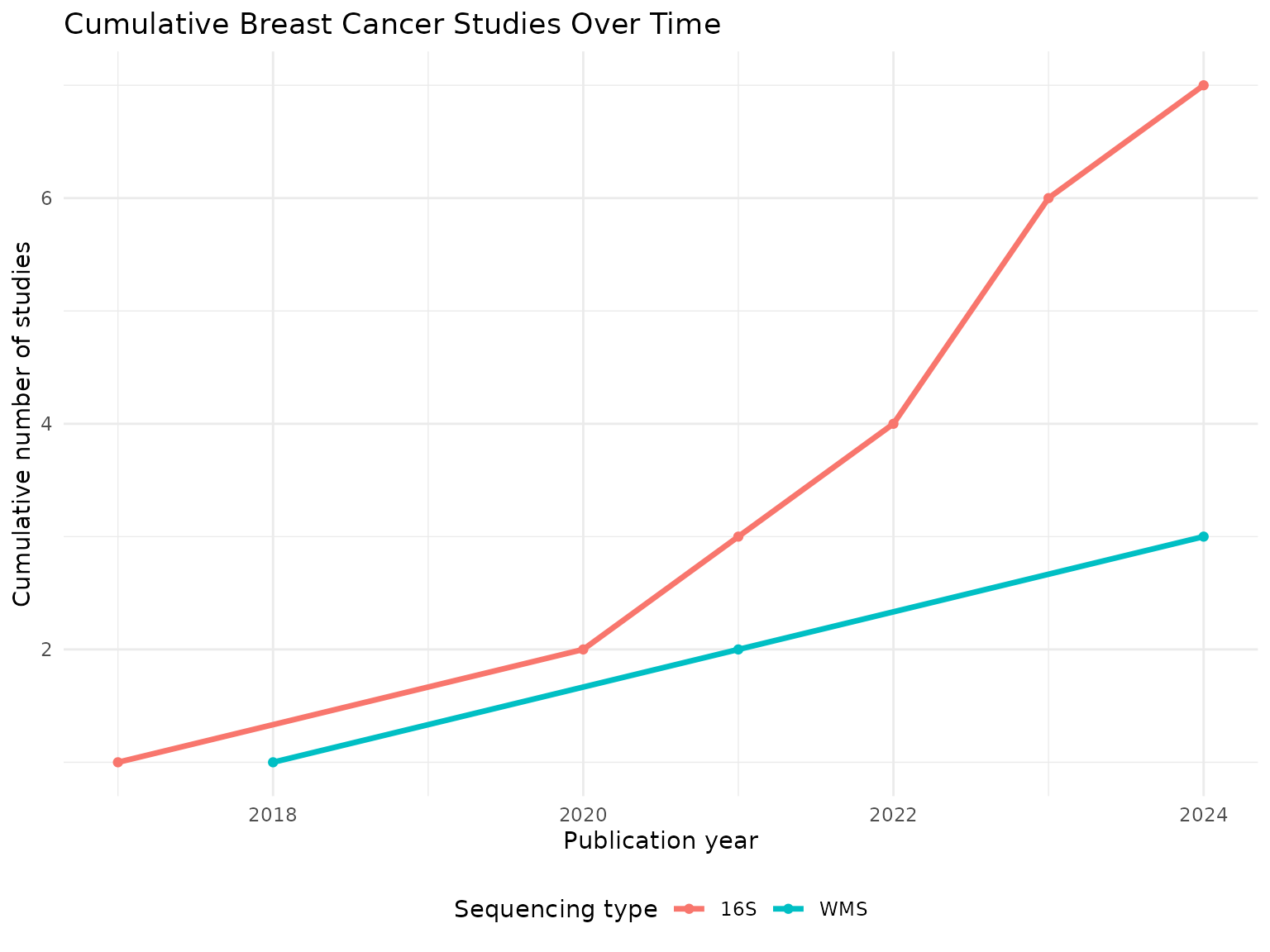

Taxonomic Summary

taxa.table <- createTaxonTable(breast_dat)
knitr::kable(head(taxa.table, 20))

Taxon Name	Taxonomic Level	total_signatures	increased_signatures	decreased_signatures	Binomial Test pval
Bacteroides	genus	6	4	2	0.69
Eggerthella	genus	5	3	2	1.00
Streptococcus	genus	5	1	4	0.37
Oscillospiraceae	family	5	3	2	1.00
Collinsella aerofaciens	species	4	0	4	0.12
Ruminococcus	genus	4	1	3	0.63
Lachnospiraceae	family	4	1	3	0.63
Anaerostipes	genus	4	0	4	0.12
Acidaminococcus	genus	4	3	1	0.63
Dialister	genus	4	0	4	0.12

Split by Sequencing Type

breast.wms <- breast_dat %>% filter(`Sequencing type` == "WMS")
breast.16s <- breast_dat %>% filter(`Sequencing type` == "16S")

cat("WMS  - signatures:", nrow(breast.wms), "| studies:", n_distinct(breast.wms$PMID), "\n")

## WMS  - signatures: 9 | studies: 3

cat("16S  - signatures:", nrow(breast.16s), "| studies:", n_distinct(breast.16s$PMID), "\n")

## 16S  - signatures: 34 | studies: 7

Long-Format Taxon Table Setup

sigs.breast <- bugsigdbr::getSignatures(breast_dat, tax.id.type = "taxname")

# Also pull a broader copy for cross-condition reference background mapping
sigs.all <- bugsigdbr::getSignatures(dat, tax.id.type = "taxname")

taxon.long <- purrr::map_dfr(seq_along(sigs.all), function(i) {
  taxa <- sigs.all[[i]]
  if (length(taxa) == 0) return(NULL)
  tibble::tibble(sig_id = i, taxon = taxa)
}) %>%
  left_join(
    dat %>%
      mutate(sig_id = row_number()) %>%
      select(sig_id, PMID, Condition, `Sequencing type`, `Abundance in Group 1`),
    by = "sig_id"
  ) %>%
  rename(direction = `Abundance in Group 1`)

cat("Long-format table successfully built with", nrow(taxon.long), "rows.\n")

## Long-format table successfully built with 58971 rows.

knitr::kable(head(taxon.long), caption = "Preview of the Structured Long-Format Taxon Table")

Preview of the Structured Long-Format Taxon Table
sig_id	taxon	PMID	Condition	Sequencing type	direction
1	Acinetobacter johnsonii	NA	Obesity	WMS	increased
1	Anaerostipes	NA	Obesity	WMS	increased
1	Anaerostipes caccae	NA	Obesity	WMS	increased
1	Brachyspira hyodysenteriae	NA	Obesity	WMS	increased
1	Coprococcus	NA	Obesity	WMS	increased
1	Allocoprococcus comes	NA	Obesity	WMS	increased

Taxon Frequency Across Studies

taxon.freq <- taxon.long %>%
  filter(Condition %in% breast_terms) %>%
  distinct(PMID, taxon, direction) %>%
  count(taxon, direction, name = "n_studies") %>%
  group_by(taxon) %>%
  mutate(total_studies = sum(n_studies)) %>%
  ungroup() %>%
  arrange(desc(total_studies))

n_distinct(taxon.freq$taxon)

## [1] 294

taxon.freq %>%
  distinct(taxon, total_studies) %>%
  slice_max(total_studies, n = 15) %>%
  knitr::kable()

taxon	total_studies
Lachnospiraceae	4
Prevotella	4
Anaerostipes	3
Bacillota	3
Mediterraneibacter torques	3
Alistipes	2
Bacteroides	2
Bacteroidota	2
Blautia	2
Dialister	2
Dorea longicatena	2
Eggerthella	2
Helotiales	2
Methanobrevibacter	2
Prevotellaceae	2
Saccharomyces	2
Saccharomycetaceae	2
Saccharomycetales	2
Saccharomycetes	2
Trichosporonaceae	2
Trichosporonales	2
[Clostridium] leptum	2
uncultured Oscillospiraceae bacterium	2

Core Consensus Signature

concordance <- taxon.long %>%
  filter(Condition %in% breast_terms) %>%
  distinct(PMID, taxon, direction) %>%
  group_by(taxon) %>%
  summarise(
    n_studies       = n_distinct(PMID),
    n_increased     = sum(direction == "increased"),
    n_decreased     = sum(direction == "decreased"),
    concordance_pct = round(max(n_increased, n_decreased) / n_studies * 100, 1),
    majority_dir    = if_else(n_increased >= n_decreased, "increased", "decreased"),
    .groups = "drop"
  ) %>%
  arrange(desc(n_studies), desc(concordance_pct))

# Standard threshold (matching the General analysis): >=3 studies, >=75% concordance.
# If this returns very few/zero rows given the smaller sample size here, consider
# loosening to >=2 studies / >=70% concordance, as was done for Cervical Cancer -
# and note that deviation explicitly in the Discussion section if you do.
core.sig <- concordance %>%
  filter(n_studies >= 3, concordance_pct >= 75) %>%
  arrange(majority_dir, desc(n_studies))

nrow(core.sig)

## [1] 0

knitr::kable(core.sig)

taxon	n_studies	n_increased	n_decreased	concordance_pct	majority_dir

Core Signature Visualisation

if (nrow(core.sig) > 0) {
  core.sig %>%
    group_by(majority_dir) %>%
    slice_max(n_studies, n = 15, with_ties = FALSE) %>%
    ungroup() %>%
    mutate(
      direction_label = if_else(majority_dir == "increased", "Increased", "Decreased"),
      taxon_label = paste0(str_wrap(taxon, width = 28), " (", n_studies, ")")
    ) %>%
    ggplot(aes(x = reorder(taxon_label, n_studies), y = n_studies, fill = direction_label)) +
    geom_col(width = 0.7) +
    geom_text(aes(label = paste0(concordance_pct, "%")), hjust = -0.15, size = 3.3) +
    coord_flip(clip = "off") +
    facet_wrap(~direction_label, scales = "free_y", ncol = 1) +
    scale_fill_manual(values = c("Increased" = "#FFB7D5", "Decreased" = "#FDF6E2")) +
    scale_y_continuous(expand = expansion(mult = c(0, 0.35))) +
    labs(
      title = "Core Breast Cancer Consensus Signature",
      x = NULL, y = "Number of independent studies", fill = NULL
    ) +
    theme_minimal(base_size = 12) +
    theme(legend.position = "none", plot.title = element_text(face = "bold"))
} else {
  cat("No taxa met the core-signature threshold at this sample size.")
}

## No taxa met the core-signature threshold at this sample size.

WMS vs 16S Concordance

dir.by.platform <- taxon.long %>%
  filter(Condition %in% breast_terms) %>%
  filter(`Sequencing type` %in% c("WMS", "16S")) %>%
  distinct(PMID, taxon, direction, `Sequencing type`) %>%
  count(taxon, `Sequencing type`, direction, name = "n_studies") %>%
  group_by(taxon, `Sequencing type`) %>%
  slice_max(n_studies, n = 1, with_ties = FALSE) %>%
  ungroup() %>%
  select(taxon, `Sequencing type`, majority_dir = direction)

platform.compare <- dir.by.platform %>%
  pivot_wider(names_from = `Sequencing type`, values_from = majority_dir) %>%
  filter(!is.na(WMS), !is.na(`16S`)) %>%
  rename(dir_WMS = WMS, dir_16S = `16S`) %>%
  mutate(agree = dir_WMS == dir_16S)

nrow(platform.compare)

## [1] 8

if (nrow(platform.compare) > 0) {
  sum(platform.compare$agree)
  round(100 * mean(platform.compare$agree), 1)
  knitr::kable(platform.compare)
} else {
  cat("No taxa reported by both WMS and 16S in this breast-cancer dataset.")
}

taxon	dir_16S	dir_WMS	agree
Bacillota	increased	decreased	FALSE
Bacteroides	increased	increased	TRUE
Bacteroidota	decreased	increased	FALSE
Dialister	increased	decreased	FALSE
Dorea longicatena	increased	increased	TRUE
Mediterraneibacter torques	decreased	increased	FALSE
Prevotella	decreased	decreased	TRUE
[Clostridium] leptum	increased	increased	TRUE

Taxon Enrichment Analysis

n.universe <- n_distinct(taxon.long %>% filter(Condition %in% breast_terms) %>% pull(taxon))
n.sigs     <- length(sigs.breast)

enrichment.df <- taxon.freq %>%
  distinct(taxon, total_studies) %>%
  mutate(
    observed         = total_studies,
    expected         = n.sigs / n.universe,
    enrichment_ratio = observed / expected,
    log2_enrichment  = log2(enrichment_ratio),
    p_value = purrr::map_dbl(observed, ~ binom.test(
      x = .x, n = n.sigs, p = 1 / n.universe, alternative = "greater"
    )$p.value),
    p_adj = p.adjust(p_value, method = "BH")
  ) %>%
  arrange(p_adj, desc(log2_enrichment))

sum(enrichment.df$p_adj < 0.05)

## [1] 5

knitr::kable(head(enrichment.df, 15))

taxon	total_studies	observed	expected	enrichment_ratio	log2_enrichment	p_value	p_adj
Lachnospiraceae	4	4	0.1462585	27.34884	4.773408	0.0000149	0.0021839
Prevotella	4	4	0.1462585	27.34884	4.773408	0.0000149	0.0021839
Anaerostipes	3	3	0.1462585	20.51163	4.358370	0.0004386	0.0257906
Bacillota	3	3	0.1462585	20.51163	4.358370	0.0004386	0.0257906
Mediterraneibacter torques	3	3	0.1462585	20.51163	4.358370	0.0004386	0.0257906
Alistipes	2	2	0.1462585	13.67442	3.773408	0.0095236	0.1217367
Bacteroides	2	2	0.1462585	13.67442	3.773408	0.0095236	0.1217367
Bacteroidota	2	2	0.1462585	13.67442	3.773408	0.0095236	0.1217367
Blautia	2	2	0.1462585	13.67442	3.773408	0.0095236	0.1217367
Dialister	2	2	0.1462585	13.67442	3.773408	0.0095236	0.1217367
Dorea longicatena	2	2	0.1462585	13.67442	3.773408	0.0095236	0.1217367
Eggerthella	2	2	0.1462585	13.67442	3.773408	0.0095236	0.1217367
Helotiales	2	2	0.1462585	13.67442	3.773408	0.0095236	0.1217367
Methanobrevibacter	2	2	0.1462585	13.67442	3.773408	0.0095236	0.1217367
Prevotellaceae	2	2	0.1462585	13.67442	3.773408	0.0095236	0.1217367

Monte Carlo Critical N

siglengths <- lengths(breast_dat$`MetaPhlAn taxon names`)

criticalN <- getCriticalN(
  relevant.sigs = breast_dat$`MetaPhlAn taxon names`,
  siglengths = siglengths
)

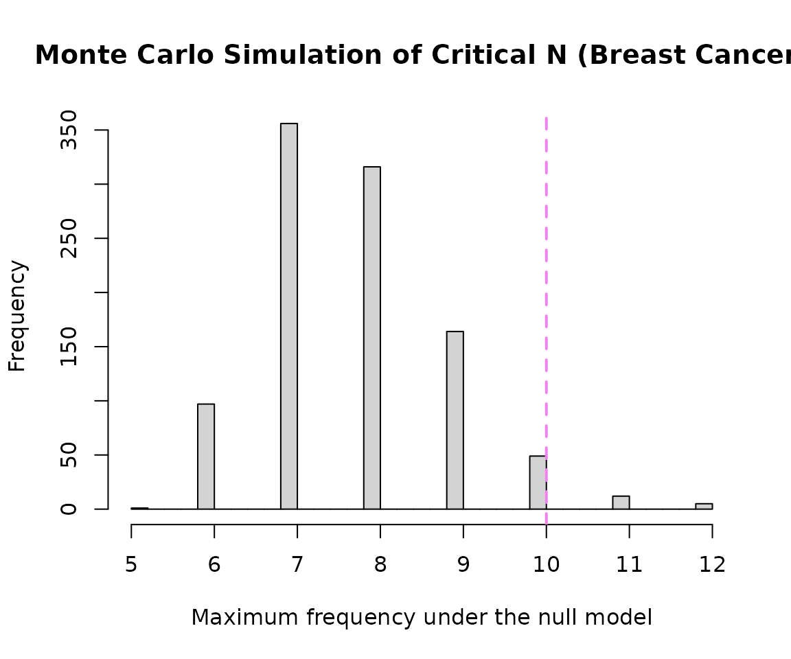
criticalN

## $critical_n
## 95% 
##  10 
## 
## $ci_lower
## 2.5% 
##   10 
## 
## $ci_upper
## 97.5% 
##    10 
## 
## $simulated_values
##    [1]  7  7  7  8  7  8  7  8  7  7  7  6  9  7  7  7  7  7  9  7  8  6  9  8
##   [25]  6  8  8  8  6  8  8  8  7  6  7  8  6  6  9  7  7  7  8  9  6  9  8  9
##   [49]  7  7  8  8  7  8  7  6  7  7  8  7  8  9  8  9  9  9  8  8  7  7  9  8
##   [73]  8  6  8  8  8  7  8  9  8  8  7  9  8  7  9  6  7 10  7  6  7  7  8  7
##   [97]  8 10  7  7  7  7  7  8  6  8  8  7  7  7  8  8  8  8  7  8  7  8  8  9
##  [121]  6  7  6  9  5  8  7  7  9  8 11  8  9  7  6  7  7  8  9  9  8  7  7  9
##  [145]  6  8  7  6  8  7  7  7 11  7  6  8 10  9  8  8  8  9  8  7  9  8  9  7
##  [169]  9  8  7  9  8  8  7 10  7  8  9  7  8  8  8  6  7  7  8  8  8  9  8  8
##  [193]  9 12  7  9  9  7  9  6  7  8  9  7  8  8 10  8  6  8  7  8  9  7  7  7
##  [217]  7  8  8 10  7  7  7  7  8  8  8 10  8  7  9  9  6  8  9  8 10  9  7  8
##  [241]  9  8  9  9  7  8  7  6  8  9  7 10  8  7  7  8 10  7  8  7  8  8  8  6
##  [265]  7  8  7  8  9 11  9  8  9  7  9  8  8  8  9  7  7  7  8  7  7  8  6 12
##  [289]  7  9  9  7  7  8  6  8  7  9  7  9  7 10  9  8  7 11  7  7  8  9  9  7
##  [313]  9 11  7  9 10  8  6  8  8  8  7  7  8  7  9 10  7  9  7  8  7  7  7  8
##  [337] 10 10  8  8 10  9  9  6  7  7  6  8  6  8  9  8  7  9  7  7  6  7 10  6
##  [361]  7  8  9  8  9  7  9  7  7  8  9  8  7  8  7  8  7  9  8  9  7  8  7  7
##  [385]  8 11  9  7  7  7  9  7  9  8  7  7  7  9  7  7  9  7  6 10  7  8  8  7
##  [409]  7  7  6  8  8  8 11  6 10  6  8  7  7  7  9  8  6 10  6  8  8 10  7 11
##  [433]  8  7  6  7  7  8  8  8  8  8  8  7  7 10  7  8  8  7  9  7  6 10  7  7
##  [457]  7  7  6  8  8  7  8  8  7  8  7  9  8  7  7  7  8  6  7  9 10  7  7  7
##  [481]  8  7  9  7 10  8  8  8  8  7  7  8  8  9  7  7  6  9  6  8  8  7  9  6
##  [505]  8  9  8  7  6  7  8  7 12  9  8  7  8  7  7  8  6  9  7  7  8  9  6  9
##  [529]  8  6  8  8  7  9  8  7  7  7  7  9  8  7  8  7  9  7  7  8  9  7  6  7
##  [553]  7  7  9  7  7  7  7 10  8  8  9  7  7 10  8  9  7  7  7  8  9  9  7  6
##  [577]  6  8  7  6  7  9  7  8  9  7  7  7  8  9  9 10  8  7  7 10  7  9  7  7
##  [601]  9  7 11  7  9  6  8  7  9  8  6  8  9  8  7  9  6  6  9  6  8  8  7  8
##  [625] 11  6  9  8  7  8  8  9  8  7  7  6  8  6  8  7  7  9  6  7 12  8  7  8
##  [649]  8  8  9  8  7  8  8  7  8  8  8  9  8  7  8  8  6  7  7  8  7  6  9  8
##  [673]  7  8  7  6  8  7  9  8  7  8 10  8  7  7  6  7  9  8 12  8  7  8  7  7
##  [697]  6  7  8  7  8  7  6  7  8  7  8  6  7  7  8  7  9  7  7  7  9  7  7  7
##  [721]  8  7  8  6  7  9  8  7  9  9  8  9  6  7  7  9  8  7  7  7  9  8 10  8
##  [745]  7  8  8  7  8  7 10  7  7  7  9  7 10  8  9  9  7 10  8  8  6  8  8  8
##  [769]  8  7  7  7  8  9 10  8  8  7  8  8  9  8  6  7  8  8  9  8  9  9  6  9
##  [793]  6 10  7 10  9  7  9  9  7  6  7  8  8  7  8  7  7  7  7  6  7  7  7  9
##  [817] 10  8  8  8  7  9  9  9  8  8 10  8  8  8  7  9  8  7  6  6  8  9  8  8
##  [841]  8  8  7  8  6  9  8  7  9 10  9  8  9  7  6  7  7  6  8  7  9  9  7 10
##  [865]  8  8  8  8  8  7 10  8  8 11  8  7  6  8  8 10  8  7  7  8  7  7 10  9
##  [889]  7  6  7  7  7  7  6  7  8  7  8  8  8  8  9  7  7  7  7  8  8  8  7  9
##  [913]  8  8  6  8 11  7  8  8  8  7  8  7  6  7  9  7 10  6  8  7  7  7 10  8
##  [937]  7  8  6  7  6  9 10  6  7  9  8  7  7  8  8  9  7  8  9  7  7  8  9  7
##  [961]  8  9  9  9  8  7  8  6 10  7  8  7  9  7  7  7  9  8  8  7  8  6  6  8
##  [985]  9 10  7  6  7  8  9  7  7  8  7  7  7  7  6  8
## 
## $alpha
## [1] 0.05
## 
## $quantile_label
## [1] "95th percentile"

hist(
  criticalN$simulated_values,
  breaks = 30,
  main = "Monte Carlo Simulation of Critical N (Breast Cancer)",
  xlab = "Maximum frequency under the null model"
)

abline(
  v = criticalN$critical_n,
  col = "violet",
  lwd = 2,
  lty = 2
)

Cross-Condition Taxa Overlap Analysis

This section explores whether the taxa altered in breast cancer are unique to breast tissue/tumor microenvironment changes or represent shared dysbiosis markers also seen across other women’s health conditions.

breast_taxa <- taxon.long %>%
  filter(Condition %in% breast_terms) %>%
  distinct(taxon) %>%
  pull(taxon)

shared_taxa_counts <- taxon.long %>%
  filter(taxon %in% breast_taxa) %>%
  group_by(taxon) %>%
  summarise(
    total_womens_health_studies = n_distinct(PMID),
    distinct_conditions_linked = n_distinct(Condition),
    top_other_conditions = paste(
      head(setdiff(unique(Condition), breast_terms), 3),
      collapse = ", "
    ),
    .groups = "drop"
  ) %>%
  arrange(desc(distinct_conditions_linked))

shared_taxa_counts %>%
  slice_max(distinct_conditions_linked, n = 20, with_ties = FALSE) %>%
  knitr::kable(
    caption = "Top Breast-Cancer-Associated Taxa and Their Links to Other Women's Health Conditions",
    col.names = c("Taxon Name", "Total WH Studies", "Total Distinct Conditions", "Other Conditions it Often Appears In")
  )

Top Breast-Cancer-Associated Taxa and Their Links to Other Women’s Health Conditions
Taxon Name	Total WH Studies	Total Distinct Conditions	Other Conditions it Often Appears In
Prevotella	354	211	Illness severity status, Antimicrobial agent, Obesity
Lactobacillus	335	201	Antimicrobial agent, Oxygen, Illness severity status
Bacteroides	345	199	Autism, Autoimmune disease, Obesity
Lachnospiraceae	331	199	Autoimmune disease, Smoking behavior, Irritable bowel syndrome
Bacillota	313	190	Type II diabetes mellitus, Autism, Autoimmune disease
Faecalibacterium	278	183	Obesity, Autoimmune disease, Irritable bowel syndrome
Bifidobacterium	275	177	Food allergy, Irritable bowel syndrome, Autism
Clostridium	258	175	Irritable bowel syndrome, Autism, Autoimmune disease
Actinomycetota	265	171	Autism, Ethnic group,Place of residence measurement, Ulcerative colitis
Pseudomonadota	241	166	Autism, Autoimmune disease, Ethnic group,Place of residence measurement
Roseburia	228	165	Autoimmune disease, Smoking behavior, Irritable bowel syndrome
Blautia	246	164	Autoimmune disease, Irritable bowel syndrome, Colorectal cancer
Veillonella	241	161	Obesity, Antimicrobial agent, Oxygen
Bacteroidota	247	158	Autism, Autoimmune disease, Irritable bowel syndrome
Enterobacteriaceae	213	155	Autoimmune disease, Irritable bowel syndrome, Sampling site
Alistipes	198	148	Autoimmune disease, Irritable bowel syndrome, Colorectal cancer
Ruminococcus	218	147	Autism, Autoimmune disease, Irritable bowel syndrome
Parabacteroides	208	145	Autism, Autoimmune disease, Irritable bowel syndrome
Clostridia	188	140	Type II diabetes mellitus, Autoimmune disease, Colorectal carcinoma
Lactobacillaceae	194	134	Autoimmune disease, Antimicrobial agent, Psoriasis

Shared Dysbiosis Visualisation

top_shared_taxa <- shared_taxa_counts %>%
  filter(distinct_conditions_linked > 1) %>%
  slice_max(total_womens_health_studies, n = 15, with_ties = FALSE) %>%
  pull(taxon)

if (length(top_shared_taxa) > 0) {
  taxon.long %>%
    filter(taxon %in% top_shared_taxa) %>%
    mutate(Condition_Group = if_else(Condition %in% breast_terms, "Breast Cancer", Condition)) %>%
    count(taxon, Condition_Group) %>%
    ggplot(aes(x = reorder(taxon, n), y = n, fill = Condition_Group)) +
    geom_col() +
    coord_flip() +
    labs(
      title = "Breast Cancer Taxa Active in Other Conditions",
      subtitle = "Tracking where prominent breast-cancer-associated microbes show up elsewhere",
      x = NULL, y = "Total Signature Mentions", fill = "Condition Group"
    ) +
    theme_minimal(base_size = 11) +
    theme(legend.position = "right")
}

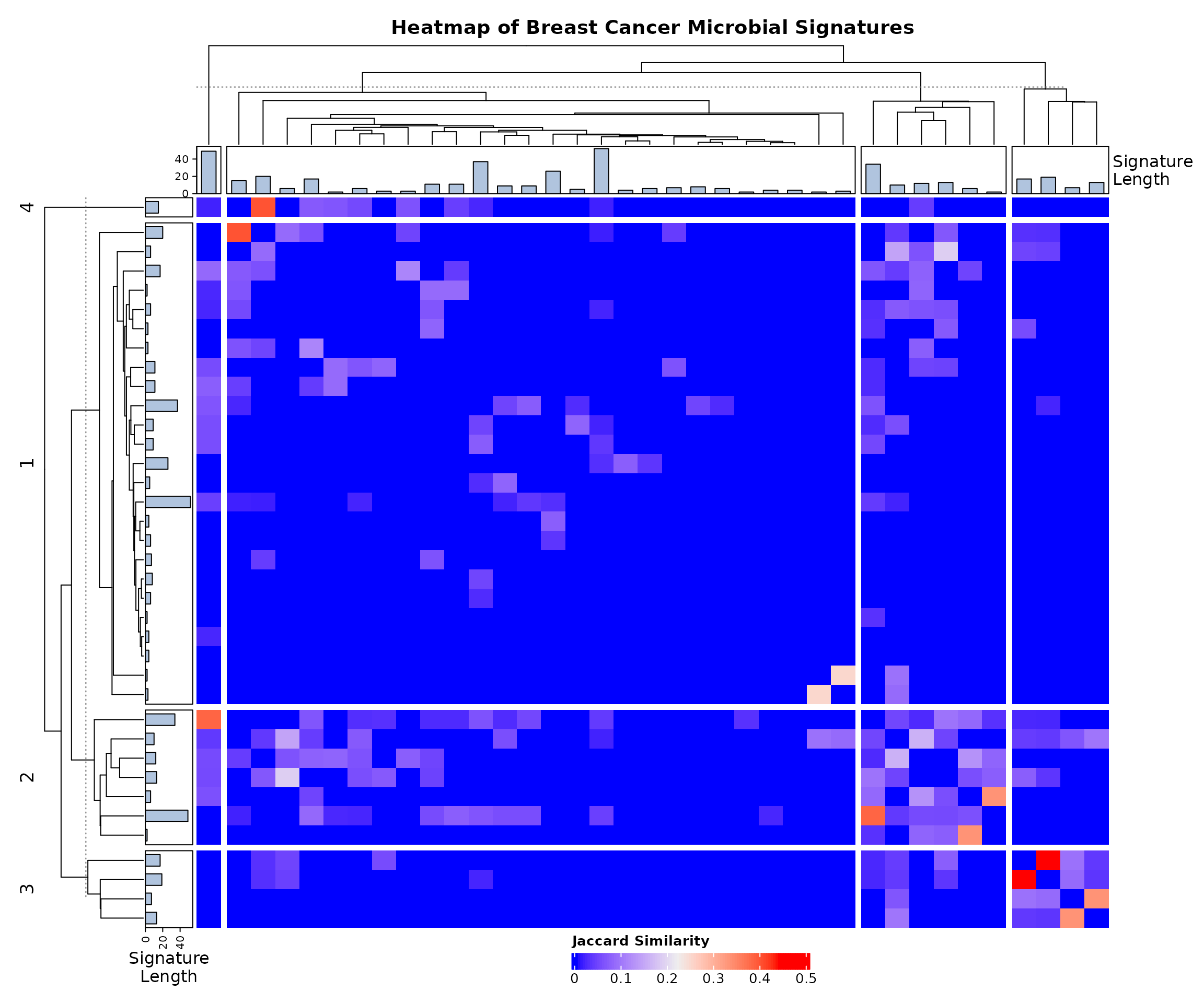
Signature Similarity and Heatmap

allsigs <- bugsigdbr::getSignatures(breast_dat, tax.id.type = "taxname")
allsigs <- allsigs[sapply(allsigs, length) > 1]

if (length(allsigs) > 1) {
  jmat <- BugSigDBStats::calcJaccardSimilarity(allsigs)
  siglengths <- sapply(allsigs, length)

  ha <- HeatmapAnnotation(
    `Signature\nLength` = anno_barplot(siglengths, gp = gpar(fill = "#B0C4DE"), height = unit(1.2, "cm"))
  )
  hr <- rowAnnotation(
    `Signature\nLength` = anno_barplot(siglengths, gp = gpar(fill = "#B0C4DE"), width = unit(1.2, "cm"))
  )

  hm <- Heatmap(
    jmat,
    top_annotation = ha,
    left_annotation = hr,
    show_row_names = FALSE,
    show_column_names = FALSE,

    row_km = 4,
    column_km = 4,
    row_gap = unit(1.5, "mm"),
    column_gap = unit(1.5, "mm"),

    row_dend_width = unit(2.5, "cm"),
    column_dend_height = unit(2.5, "cm"),

    column_title = "Heatmap of Breast Cancer Microbial Signatures",
    column_title_gp = gpar(fontsize = 14, fontface = "bold"),
    heatmap_legend_param = list(
      title = "Jaccard Similarity",
      direction = "horizontal",
      legend_width = unit(6, "cm")
    )
  )

  draw(hm, heatmap_legend_side = "bottom", padding = unit(c(5, 5, 5, 5), "mm"))

  png(filename = "BreastCancer_heatmap.png", width = 12, height = 10, units = "in", res = 300)
  draw(hm, heatmap_legend_side = "bottom", padding = unit(c(5, 5, 5, 5), "mm"))
  dev.off()
}

## agg_png 
##       2

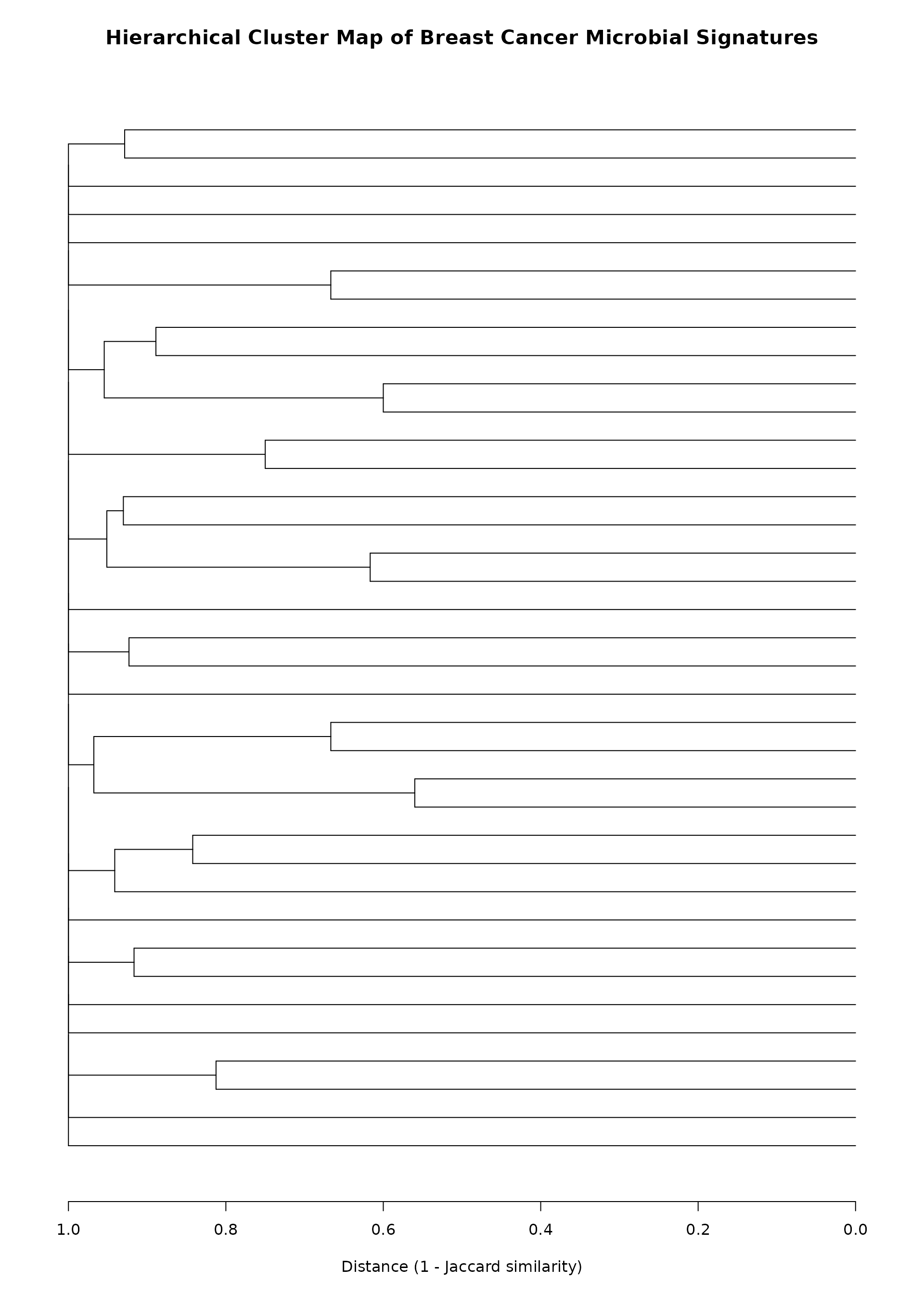
Dendrogram

if (exists("jmat") && nrow(jmat) > 1) {
  hc <- hclust(as.dist(1 - jmat))
  dend <- as.dendrogram(hc)

  par(mar = c(5, 2, 4, 2))

  plot(
    dend,
    horiz = TRUE,
    leaflab = "none",
    main = "Hierarchical Cluster Map of Breast Cancer Microbial Signatures",
    xlab = "Distance (1 - Jaccard similarity)",
    cex.main = 1.3,
    lwd = 0.8
  )
}

Condition-Specific Analysis with Cross-Condition Mapping (BugSigDB)

Sally Karimi Kinyua