Lab 3: Differential Expression and Double-Dipping

Introduction

In this lab, we will perform a differential expression analysis using the airway dataset. We will fit a Negative Binomial Generalized Linear Model (GLM) using DESeq2. Afterwards, we will demonstrate the dangers of “double-dipping”—using the data to define groups, and then testing for differences between those exact same groups on the same data.

1. The Dataset

We will use the airway package, which provides a SummarizedExperiment object containing RNA-seq data from human airway smooth muscle cells. Some cells were treated with dexamethasone (dex).

library(airway)
library(DESeq2)
library(ggplot2)

data(airway)
se <- airway
se$dex <- relevel(se$dex, ref = "untrt")

Take a look at the experimental design:

colData(se)[, c("cell", "dex")]

## DataFrame with 8 rows and 2 columns
##                cell      dex
##            <factor> <factor>
## SRR1039508  N61311     untrt
## SRR1039509  N61311     trt  
## SRR1039512  N052611    untrt
## SRR1039513  N052611    trt  
## SRR1039516  N080611    untrt
## SRR1039517  N080611    trt  
## SRR1039520  N061011    untrt
## SRR1039521  N061011    trt

2. Standard DE Analysis (The Right Way)

We will perform differential expression analysis comparing treated vs. untreated samples, controlling for the cell line.

dds <- DESeqDataSet(se, design = ~ cell + dex)
dds <- DESeq(dds)
res <- results(dds, contrast = c("dex", "trt", "untrt"))

Let’s look at the distribution of the unadjusted p-values:

hist(res$pvalue, breaks = 50, col = "grey", main = "Standard DE Analysis: trt vs untrt", xlab = "p-value")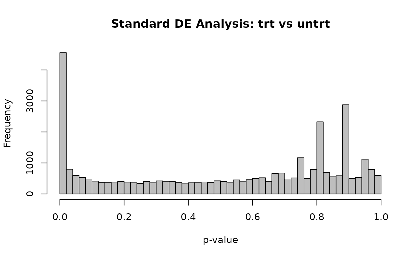

A valid p-value distribution should look roughly uniform under the null hypothesis (features with no true differential expression), with a spike near zero representing the truly differentially expressed features.

3. Demonstrating Double-Dipping (The Wrong Way)

Now we will see what happens when we use the data to define our groups before testing.

Step 3a: Permuted Labels

First, let’s establish a baseline where we know there is no biological signal. We will randomly permute the treatment labels across the samples and run the DE analysis again.

set.seed(123)
dds_perm <- dds
# Randomly shuffle the dex labels
dds_perm$dex <- sample(dds_perm$dex)
# Re-run DESeq
dds_perm <- DESeq(dds_perm, quiet = TRUE)
res_perm <- results(dds_perm, contrast = c("dex", "trt", "untrt"))

hist(res_perm$pvalue, breaks = 50, col = "grey", main = "Permuted Labels", xlab = "p-value")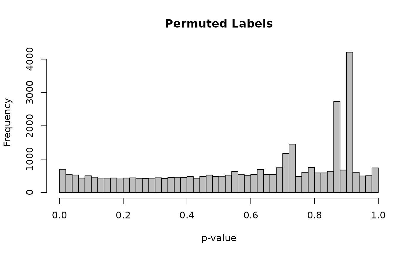

Notice that the spike near zero is gone. The distribution is approximately uniform, which is what we expect when there is no true difference between the groups.

Step 3b: Data-Driven Clustering

Now, imagine we didn’t know the treatment labels. We decide to cluster the samples based on their gene expression profiles, and then test for differential expression between the clusters we just found. This is a classic example of double-dipping.

We will provide pseudocode for how you might accomplish this. Your task is to complete the clustering step.

Recommendation: Before deciding on $k=2$ clusters, it’s often a good idea to estimate the optimal number of clusters. You can use a silhouette plot from the cluster package.

# Pseudocode for Data-Driven Clustering

# 1. Apply a variance-stabilizing transformation to the counts
# vsd <- vst(dds, blind=TRUE)

# 2. Select the top N most variable genes (e.g., top 500)
# rv <- rowVars(assay(vsd))
# select <- order(rv, decreasing=TRUE)[seq_len(500)]
# top_vsd <- assay(vsd)[select, ]

# 3. Transpose the matrix so rows are samples, columns are genes
# ...

# 4. (Optional) Create a silhouette plot to see if k=2 is reasonable
# library(cluster)
# dist_matrix <- dist(...)
# sil <- silhouette(pam(dist_matrix, k=2)$clustering, dist_matrix)
# plot(sil)

# 5. Perform k-means clustering (k=2) on the samples
# set.seed(123)
# km <- kmeans(..., centers=2)

# 6. Assign the resulting cluster labels to a new column in colData
# dds$cluster <- factor(km$cluster)

Exercise: Implement the pseudocode above to assign your samples into two clusters, cluster 1 and cluster 2, saving it as dds$cluster.

# Write your code here to assign dds$cluster

Step 3c: DE Analysis on Clusters

Once you have defined dds$cluster, run the DE analysis comparing the two clusters.

# Change the design to use our new cluster variable
design(dds) <- ~cluster
dds_clust <- DESeq(dds, quiet = TRUE)
res_clust <- results(dds_clust)

hist(res_clust$pvalue, breaks = 50, col = "grey", main = "Clustered Labels (Double Dipping)", xlab = "p-value")

4. Discussion Questions

Explain what happened in Step 3c. Why did the p-value distribution change so drastically when testing between data-driven clusters compared to testing between permuted labels?
How might you avoid this problem if you genuinely needed to discover clusters and then test for differences between them? Hint: you can give a brief summary from:

Anna Neufeld, Lucy L Gao, Joshua Popp, Alexis Battle, Daniela Witten, Inference after latent variable estimation for single-cell RNA sequencing data, Biostatistics, Volume 25, Issue 1, January 2024, Pages 270–287, https://doi.org/10.1093/biostatistics/kxac047

Quote from this paper:

“Despite this issue with double dipping, it is common practice. Monocle3 and Seurat are popular packages that each contain functions for (1) estimating latent variables such as clusters or pseudotime and (2) identifying genes that are differentially expressed across these latent variables. The vignettes for these packages perform both steps on the same data (Pliner and others, 2022; Hoffman, 2022). Consequently, the computational pipelines suggested by the package vignettes fail to control the Type 1 error rate. We demonstrate this empirically in Appendix A of the Supplementary material available at Biostatistics online.”

Applied Statistics for High-throughput Biology