Lab 4: DAGs in Data Analysis

Introduction

In this lab, we will use simulated data to demonstrate the importance of Directed Acyclic Graphs (DAGs) in guiding statistical analysis. We will see how failing to control for a confounder, or mistakenly controlling for a collider, can both lead to biased estimates of a causal effect.

We will simulate a scenario where the true causal effect of an Exposure (E) on a Disease (D) is exactly zero. However, there are two other variables present: - C (Confounder): Causes both E and D. - S (Collider): Caused by both E and D.

Let’s draw the DAG for this scenario:

library(ggdag)
library(ggplot2)

dag <- dagify(
  D ~ C,
  E ~ C,
  S ~ E + D,
  labels = c("D" = "Disease", "E" = "Exposure", "C" = "Confounder", "S" = "Collider"),
  exposure = "E",
  outcome = "D",
  coords = list(
    x = c(C = 0, E = -1, D = 1, S = 0),
    y = c(C = 1, E = 0, D = 0, S = -1)
  )
)

ggdag(dag, text = FALSE) + geom_dag_label_repel(aes(label = label)) + theme_dag()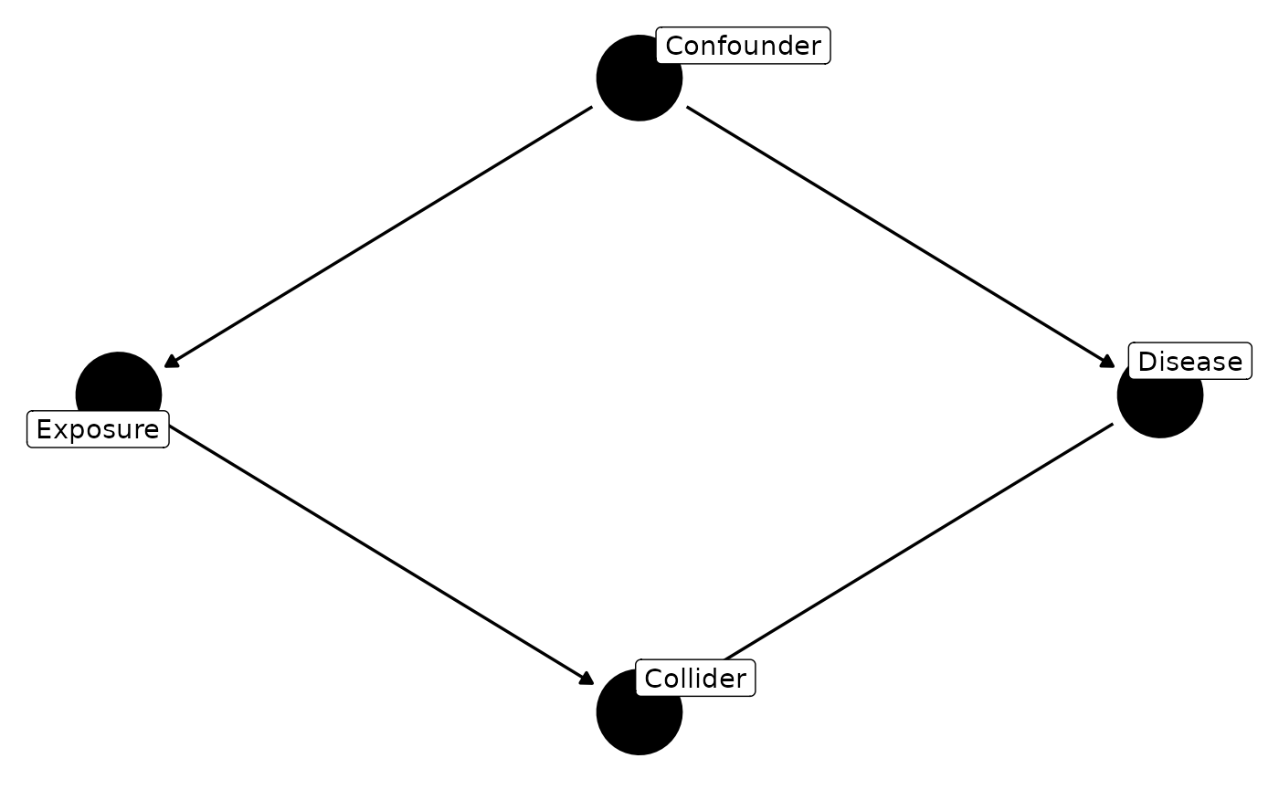

Data Simulation

We simulate 1000 observations based on the relationships defined in our DAG:

# use set.seed() if you want reproducible random numbers
N <- 1000

# 1. C is a confounder (causes E and D)
C <- rnorm(N, mean = 0, sd = 1)

# 2. E is caused by C, with some random noise
E <- 0.5 * C + rnorm(N, mean = 0, sd = 1)

# 3. D is caused by C, with some random noise.
# Crucially, the true effect of E on D is 0.
D <- 0.5 * C + 0 * E + rnorm(N, mean = 0, sd = 1)

# 4. S is a collider (caused by both E and D)
S <- 0.5 * E + 0.5 * D + rnorm(N, mean = 0, sd = 1)

# Combine into a dataframe
df <- data.frame(E, D, C, S)

Data Analysis

We want to estimate the causal effect of E on D. We know the true effect is 0. Let’s see what happens under different modeling choices.

1. A Biased Model: Failing to Control for the Confounder

If we simply regress D on E without controlling for the confounder C, the path E <- C -> D remains open. This “backdoor path” creates a spurious association between E and D.

summary(lm(D ~ E, data = df))

## 
## Call:
## lm(formula = D ~ E, data = df)
## 
## Residuals:
##     Min      1Q  Median      3Q     Max 
## -3.1135 -0.7472 -0.0034  0.7150  3.1806 
## 
## Coefficients:
##             Estimate Std. Error t value Pr(>|t|)    
## (Intercept)  0.04558    0.03527   1.292    0.197    
## E            0.23263    0.03186   7.302 5.77e-13 ***
## ---
## Signif. codes:  0 '***' 0.001 '**' 0.01 '*' 0.05 '.' 0.1 ' ' 1
## 
## Residual standard error: 1.115 on 998 degrees of freedom
## Multiple R-squared:  0.05072,    Adjusted R-squared:  0.04977 
## F-statistic: 53.33 on 1 and 998 DF,  p-value: 5.767e-13

Notice that the coefficient for E is statistically significant and positive, even though the true effect is 0!

Now the coefficient for E is very close to 0 and not statistically significant. We successfully recovered the true effect.

2. Another Biased Model: Improperly Controlling for the Collider

What if we decide to throw all available variables into the model, controlling for both C and S?

By conditioning on a collider (S), we open up a new non-causal path between E and D. This introduces “collider bias”.

summary(lm(D ~ E + C + S, data = df))

## 
## Call:
## lm(formula = D ~ E + C + S, data = df)
## 
## Residuals:
##     Min      1Q  Median      3Q     Max 
## -3.0798 -0.6319 -0.0010  0.6348  3.2990 
## 
## Coefficients:
##             Estimate Std. Error t value Pr(>|t|)    
## (Intercept)  0.04833    0.02831   1.707   0.0881 .  
## E           -0.18926    0.03126  -6.055 1.99e-09 ***
## C            0.41459    0.03392  12.221  < 2e-16 ***
## S            0.40434    0.02570  15.734  < 2e-16 ***
## ---
## Signif. codes:  0 '***' 0.001 '**' 0.01 '*' 0.05 '.' 0.1 ' ' 1
## 
## Residual standard error: 0.895 on 996 degrees of freedom
## Multiple R-squared:  0.3899, Adjusted R-squared:  0.3881 
## F-statistic: 212.2 on 3 and 996 DF,  p-value: < 2.2e-16

By controlling for the collider S, the coefficient for E becomes statistically significant and negative. We have introduced bias by over-adjusting!

2. The Unbiased Model: Properly Controlling for the Confounder

To get an unbiased estimate of the effect of E on D, we must block the backdoor path by controlling for the confounder C. We also must not control for the collider S.

Try this yourself, show your code and output, and let me know what you find. What happens when you simply “control for everything”?

Exercise: The Importance of Visualization and Diagnostics

We have prepared four datasets (Dataset A, B, C, and D). For each dataset, you will analyze the relationship between x and y.

dataset_A <- data.frame(x = anscombe$x1, y = anscombe$y1)
dataset_B <- data.frame(x = anscombe$x2, y = anscombe$y2)
dataset_C <- data.frame(x = anscombe$x3, y = anscombe$y3)
dataset_D <- data.frame(x = anscombe$x4, y = anscombe$y4)

Task 1: Linear Models Fit a simple linear regression model (lm(y ~ x)) for each of the four datasets. Use summary() to examine the output of each model. - What do you notice about the coefficient estimates, R-squared values, and p-values across the four models? - Comment on your findings.

Task 2: Visualization Create a scatterplot (plot(x, y)) for each of the four datasets. - Do the scatterplots look the way you expected based on the summary() output in Task 1? - Comment on any differences between the datasets.

Task 3: Diagnostics Run standard regression diagnostics (plot(model)) on each of your four fitted linear models from Task 1. - Comment on anything that stands out to you in the diagnostic plots. - Which dataset is actually appropriate for simple linear regression?